

- Share
Federal Funds Rates Based on Seven Simple Monetary Policy Rules
Monetary policymakers often use simple monetary policy rules, like the Taylor rule, as an input into their decision-making. However, there are many different simple rules, and there is no agreement on a single “best” rule. We look at the federal funds rates coming from seven simple rules and three economic forecasts to investigate the range of results that can be produced. While there are some commonalities, we document that the differences in the federal funds rates suggested by the rules can be quite pronounced.


The views authors express in Economic Commentary are theirs and not necessarily those of the Federal Reserve Bank of Cleveland or the Board of Governors of the Federal Reserve System. The series editor is Tasia Hane. This paper and its data are subject to revision; please visit clevelandfed.org for updates.
Simple monetary policy rules provide a relationship between the central bank’s policy rate and a relatively small number of indicators on real economic activity and inflation. Since the early 1990s, a large academic research literature has developed around the creation and testing of simple monetary policy rules. At the same time, policymakers have come to often look at a variety of monetary policy rules as an input into their decision-making and as a means of communicating the rationale of those decisions to the public (see, e.g., Yellen 2012, Meyer 2002, Plosser 2014, and Asso et al. 2010).
In this Commentary, we look at a range of simple monetary policy rules and their implications for the federal funds rate based on multiple forecasts. Examining a variety of rules is helpful because there is no agreement on a single “best” rule. At the same time, it is useful to consider multiple forecasts for the current state of the economy and how the economy is likely to evolve going forward, because the future is inherently uncertain and our ability to measure present economic circumstances is imperfect.
This exercise reveals some commonalities but also quite pronounced differences across the simple policy rules we consider. In a 2012 speech, then-Vice Chair Janet Yellen noted that “a wide variety of simple rules have been proposed in the academic literature, and their policy implications can differ significantly depending on the particular specification.” In looking across the rules and forecasts over the next two years, the differences between the implied federal funds rates at the 75th percentile and the 25th percentile range from 0.9 to 1.4 percentage points. Even for a single forecast, some of the differences among the rules are as large as three percentage points.
The General Form of Many Simple Monetary Policy Rules
Simple monetary policy rules often take the general form:
it = ρit − 1 + (1 − ρ)[r* + πt + α(inflation gap) + β(activity gap)].
In this rule, it is the central bank’s policy rate, such as the federal funds rate in the United States, at time t. The variable r* refers to the equilibrium real interest rate, which within the above rule can be thought of as the long-run federal funds rate adjusted for inflation. The inflation rate is πt, and the inflation gap is the difference between inflation and target inflation, denoted π*. The activity gap measures the extent to which economic activity exceeds “normal” levels. Commonly, activity is measured using the output gap (the percentage difference between actual output and potential output) or the negative of the unemployment gap (the percentage point difference between the unemployment rate and the natural rate of unemployment). The coefficient ρ captures the amount of inertia in the policy rule, α determines the responsiveness of policy to the inflation gap, and β determines the responsiveness of policy to the activity gap.
In practice, the simplicity of this general monetary policy rule belies a host of complexities. Academic researchers and policymakers have not settled on the choice of the coefficients ρ, α, and β. While some policy rules use the contemporaneous values of the inflation gap and the activity gap, others assume that the current policy rate is affected by forecasts of the inflation gap and the activity gap, given that it typically takes monetary policy some time to affect inflation and real economic activity. There are also many different approaches to estimating concepts such as r*, the activity gap, and the inflation gap, and considerable uncertainty surrounds such estimates.1
Seven Simple Policy Rules
Partly as a result of the complexities laid out above, there is a large and ever-growing literature related to simple policy rules.2 Faced with a multitude of rules, we take a pragmatic approach: We select seven simple rules that have broadly representative features from this literature, and we compare and contrast the federal funds rates coming from those rules, based on current economic conditions and based on forecasts for how economic conditions may develop in the future. We lay out the seven rules we will use in this section, with formulae in table 1, and we detail the sources of the forecasts in the next section.
| 1. Taylor (1993) rule: | it = r* + πt + 0.5(πt − π*) + 0.5(output gapt) |
| 2. Core inflation in Taylor (1999) rule: | it = r* + πtCore + 0.5(πtCore− π*) + (output gapt) |
| 3. Inertial rule: | it = ρit−1 + (1 − ρ)[r* + πtCore + 0.5(πtCore− π*) + (output gapt)] |
| 4. Alternative r* rule: | it = ρit−1 + (1 − ρ)[ralt* + πtCore + 0.5(πtCore− π*) + (output gapt)] |
| 5. Forward-looking rule: | it = r* + πt+3F + 0.5(πt+3F− π*) + 0.5(output gapt) |
| 6. First-difference rule: | it = it−1 + 1.74(πt+3F − π*) − 1.19(ut−1 − ut−2) |
| 7. Low weight on output gap rule: | it = 0.91it−1 + (1 − 0.91)[r* + π* + 1.58(πt+1Q,F − π*) + 0.14(output gapt+1F)] |
The first rule is based on the policy rule suggested by Taylor (1993). Taylor (1993) fixed r* to 2 percent and used the GDP deflator as the measure of inflation. To update the rule, we make two modifications. First, given the Federal Open Market Committee’s (FOMC) Statement on Longer-Run Goals and Monetary Policy Strategy, we measure πt as inflation in the price index for personal consumption expenditures (PCE inflation) over the previous four quarters, and we set π* to 2 percent.3 Second, we account for potential changes to r* by using the median implied long-run real federal funds rate from the most recently available FOMC Summary of Economic Projections (SEP), which was 1 percent in June 2016.4
The second rule is based on a parameterization considered by Taylor (1999), in which the coefficient on the output gap is 1.0 instead of 0.5 as in the Taylor (1993) rule. Thus, policymakers are assumed to place twice the amount of weight on slack in this rule compared with the earlier rule.5 In an effort to span the range of policy rules and provide additional contrast to the first rule above, for inflation we use the four-quarter PCE inflation rate excluding food and energy, or core PCE inflation, πtCore. Core inflation measures are often used to smooth through volatility coming from food and energy price movements, in order to identify the inflation trend. Bernanke (2015) provides one perspective on the inclusion of core PCE inflation in this rule. Monetary policymakers often use versions of the Taylor (1993) and Taylor (1999) rules as benchmarks in assessing the stance of policy; see, e.g., Yellen (2012).
The third rule adds inertia, such that the funds rate does not adjust immediately to the value of the Taylor (1999) rule with core PCE inflation, but rather moves there slowly over time. Empirical estimates consistently find such inertial responses by central banks around the world (see, e.g., Goodhart 1999, Coibion and Gorodnichenko 2012), and theoretical and simulation-based studies also typically find that policy inertia improves economic outcomes (see, e.g., Levin et al. 2003, Woodford 2003b, Taylor and Williams 2011). As in Canzoneri et al. (2015), we set ρ = 0.8, a coefficient that is “typical of estimates that are found in the empirical literature” (p. 385).
The fourth rule captures uncertainty around r* by using an alternative estimate of it.6 Laubach and Williams (2003, 2015) estimate the natural rate of interest and find that those estimates have varied significantly through U.S. history. Their most recent estimate, which we denote ralt*, was 0.2 percent using data available on May 31, 2016.
The fifth rule incorporates forward-looking elements by replacing the realized inflation rate over the last four quarters with a forecast of PCE inflation three quarters ahead, πt+3F, as suggested by Bernanke (2010).7 Forward-looking rules begin to account for the lag between monetary policy actions and their impact on the economy, and they are also able to distinguish between transitory and persistent inflationary pressures.8 Because forecasts will encompass information that may not be available in current readings on inflation or the activity gap, forecast-based policy rules inherently bring more information to bear in the policy rule, but in an easy-to-understand and compact way (see Orphanides and Wieland 2008).
The sixth rule is a forward-looking, first-difference rule, based on Orphanides and Williams (2008, 2013). In this rule, the change—or first-difference—in the policy rate is related to a forward-looking inflation gap and the (backward-looking) change in the unemployment rate in the previous quarter, ut−1 − ut−2. This rule is notable because it omits variables that are unobservable in practice and difficult to estimate. The omission of both a long-run real funds rate r* and an activity “gap” term precludes the federal funds rates coming from this rule from being contaminated by mismeasurement of unobservable concepts.9
The seventh rule departs from the others by placing a relatively low weight on the output gap, along the lines of the literature on pure inflation-targeting.10 We base the parameters of this rule on estimates reported in Clarida et al. (2000) for a forward-looking rule with inertia, which captured U.S. monetary policy actions over the period 1982-1996. In this case, we use the forecast for quarterly annualized inflation in the next quarter, πt+1Q,F, and the forecast for the output gap in the next quarter, output gapt+1F, in the policy rule.11
Data and Forecasts
To generate the federal funds rates based on these simple policy rules, both for the current quarter and going forward, we use data and forecasts from a variety of sources. One well-known and publicly available source for economic forecasts is the quarterly Survey of Professional Forecasters (SPF) from the Federal Reserve Bank of Philadelphia; we use the median responses to ensure robustness to potential outliers. The Congressional Budget Office (CBO) is another source of publicly available forecasts, which are usually updated twice per year, in January and August. Finally, we generate forecasts from a small statistical Bayesian vector autoregression model used in previous Economic Commentaries (FRBC BVAR).12
The CBO provides detailed forecasts for PCE inflation, core PCE inflation, the unemployment rate, and the output gap over a multiyear horizon, which is all the information needed to calculate the federal funds rates implied by the seven rules, for the current quarter and for the next several years. While the SPF and the FRBC BVAR forecast PCE inflation and core PCE inflation, they only report an unemployment rate and not an output gap. However, we can construct unemployment gaps for the SPF and the FRBC BVAR.13 When working with these two forecasts, we replace the output gap in all the policy rules with the product of the unemployment gap times the inverse Okun’s coefficient as the proxy for the output gap.14
Crucially, in all cases, we take the forecast as given and then calculate the implied average federal funds rate for each quarter based on the seven simple policy rules (see also, e.g., Plosser 2014). That is, we do not model the manner in which different paths for the federal funds rate would affect the forecast—even though theory and empirical evidence suggest that higher paths for the federal funds rate would tend to slow economic activity and inflation, while lower paths for the federal funds rate would tend to increase economic activity and inflation.15
Federal Funds Rates Based on Simple Policy Rules, Today and Going Forward
With seven rules, three forecasts, and quarterly data, there are a large number of federal funds rates to share. Figure 1 provides a summary of the results using quartiles. We present the median (50th percentile) federal funds rate across all the policy rules and forecasts, along with the 25th and 75th percentiles and the maximum and minimum funds rate at each point in time. Based on data and forecasts available as of June 23, 2016, the median federal funds rate from the simple policy rules we consider rises from 0.7 percent in 2016:Q2 to 2.1 percent in 2018:Q2.16
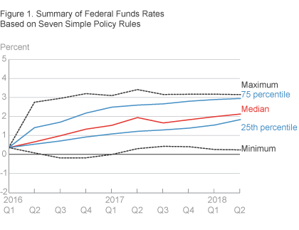
Figure 1 highlights pronounced differences among the federal funds rates coming from the various policy rules and forecasts. In the summary figure, the distance between the 75th and 25th percentiles ranges from 0.9 to 1.4 percentage points over the two-year horizon shown. Based on forecasts for the first quarter considered, 2016:Q2, the difference between the 75th and 25th percentiles is 0.9 percentage point, and the difference between the maximum and minimum federal funds rates is 2.7 percentage points.
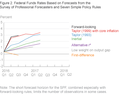
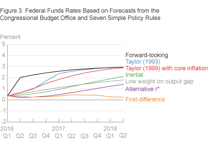
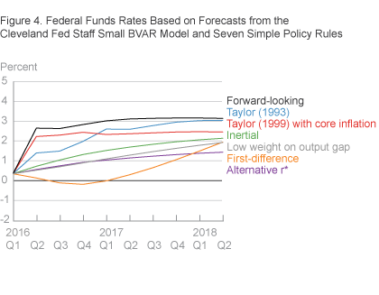
Of course, some of this variation is attributable to differences in forecasts across the three sources. Figures 2 through 4 show the federal funds rates from each simple monetary policy rule conditional on forecasts from the SPF, CBO, and FRBC BVAR, respectively. (Federal funds rates based on the SPF are limited by the SPF’s forecast horizon, which extends only one year.) Even conditional on a single forecast, we still see a wide range of implied federal funds rates: In each figure, the differences between the maximum funds rate and the minimum funds rate at a given point in time range from 1.7 to 3.1 percentage points.
Finally, while we consider multiple forecasts for inflation and real economic activity to address some of the uncertainties inherent in predicting the future and assessing the current state of the economy, it is worth noting that there is considerable uncertainty surrounding all forecasts. Thus, the summary figure likely understates the range of potential federal funds rates implied by these simple policy rules going forward, as the forecast may evolve in unexpected ways based on new incoming data.
Conclusion
This Commentary presents a relatively straightforward look at the federal funds rates coming from a range of simple monetary policy rules and forecasts. Considering a range of rules and forecasts is important, because there is not a single agreed upon “best” rule, and because there are always differing views on the economy and its future prospects. This analysis highlights some commonalities but also quite pronounced differences across simple policy rules. Even for a single forecast, some of the differences among the rules are as large as three percentage points.
Footnotes
- Uncertainty around the inflation gap typically relates to the choice of the inflation measure to include in the rule. Regarding r* and the activity gap, in addition to considerable estimation uncertainty given that these concepts are unobservable, there are multiple alternative theoretical constructs for each concept (see, e.g., Carlstrom and Stehulak 2015, and Tasci and Verbrugge 2014). Return to 1
- For one survey, see Taylor and Williams (2011). Return to 2
- With the sum of coefficients on πt of 1.5, which is greater than 1, this rule satisfies the Taylor principle, in that the real interest rate (it − πt) rises in response to increases in the inflation rate, which eventually helps to stabilize inflation. In many macroeconomic models, the policy rule coefficient on πt needs to exceed 1 in order for a unique stable equilibrium to exist (see, e.g., Woodford 2003a for a discussion). Return to 3
- The median implied long-run real federal funds rate is the median long-run federal funds rate (from figure 2 of the SEP) minus the median long-run PCE inflation rate. Carlstrom and Stehulak (2015) provide evidence of a recent decline in the long-run natural rate of interest. Return to 4
- The implications of the difference in the coefficients on the output gap have been studied elsewhere—e.g., Taylor (1999a), Meyer (2002), and Taylor and Williams (2011)—and are typically model-dependent. Return to 5
- See Clark and Kozicki (2005). Carlstrom and Fuerst (2016) find that monetary policy may achieve better outcomes if policy rules incorporate fluctuations in long-term productivity growth that proxy for a time-varying natural rate of interest. Return to 6
- Technically, we use the four-quarter rate of PCE inflation expected three quarters in the future: Within quarter t, the last observation of the price level comes from quarter t − 1, and we look at inflation four quarters ahead from that point, which is t + 3. Return to 7
- See also Ashley et al. (2014). Return to 8
- While the parameterization of the first-difference rule we consider is optimal in the context of a single model (see Orphanides and Williams 2008), first-difference rules are often robust to various forms of model uncertainty, misspecification, and learning, and can outperform optimal control policies; see, e.g., Walsh (2003), Orphanides and Williams (2008, 2013), and Tetlow (2015). Return to 9
- In fact, the coefficient on the output gap is not statistically different from zero for this case in Clarida et al. (2000). Return to 10
- While Clarida et al. (2000) estimate a relatively high value for π*, to maintain consistency with the other rules, we set π* = 2 and r* = 1 based on the FOMC’s most recent SEP. To conform to the Clarida et al. (2000) specification, the right-hand side of this rule includes π* in two locations. Return to 11
- See, e.g., Knotek et al. (2015). The Cleveland Fed staff consult a variety of forecasting models, thus this forecast does not necessarily represent the official forecast of Cleveland Fed staff or the president of the Cleveland Fed. Return to 12
- For the SPF, we take the difference between the unemployment rate and the estimate of the natural rate of unemployment (commonly called the nonaccelerating inflation rate of unemployment, or NAIRU) that the SPF updates once per year. For the FRBC BVAR, we take the difference between the unemployment rate and the long-run unemployment rate from the most recently released FOMC SEP to compute the unemployment gap. Return to 13
- We estimate Okun’s coefficient for the gap version of Okun’s law, unemployment gapt = b(output gapt), using CBO estimates for the output gap and the unemployment gap and rolling 13-year windows, as in Knotek (2007). Return to 14
- The extent to which the forecasts would endogenously differ based on alternative policy rules depends on the particular modeling assumptions employed, as well as the differences between the funds rate path implied by the policy rule and the funds rate path in the original forecast. Given the typical lags from monetary policy to real economic activity and inflation, the assumption of exogeneity of the forecast is less problematic in the near term and more problematic as the forecast horizon lengthens. Return to 15
- The three forecasts put inflation on a rising trajectory toward the FOMC’s 2 percent objective. The unemployment rate is near estimates of the natural rate, suggesting little slack in the unemployment gap, while the CBO’s output gap is negative but forecasted to gradually close by mid-2018. Return to 16
References
- Ashley, Richard, Kwok Ping Tsang, and Randal J. Verbrugge, 2014. “Frequency Dependence in a Real-Time Monetary Policy Rule,” Federal Reserve Bank of Cleveland, Working Paper, 14-30.
- Asso, Pier Francesco, George A. Kahn, and Robert Leeson, 2010. “The Taylor Rule and the Practice of Central Banking,” Federal Reserve Bank of Kansas City Research Working Paper, 10-05.
- Bernanke, Ben S., 2010. “Monetary Policy and the Housing Bubble,” Speech at the Annual Meeting of the American Economic Association, Atlanta, Georgia.
- Bernanke, Ben S., 2015. “The Taylor Rule: A Benchmark for Monetary Policy?” Ben Bernanke’s Blog, Brookings.
- Canzoneri, Matthew, Robert Cumby, and Behzad Diba, 2015. “Monetary Policy and the Natural Rate of Interest,” Journal of Money, Credit and Banking, 47(2-3): 383-414.
- Carlstrom, Charles T., and Timothy S. Fuerst, 2016. “The Natural Rate of Interest in Taylor Rules,” Federal Reserve Bank of Cleveland, Economic Commentary, 2016-01.
- Carlstrom, Charles T., and Timothy Stehulak, 2015. “The Long-Run Natural Rate of Interest,” Federal Reserve Bank of Cleveland, Economic Trends.
- Clarida, Richard, Jordi Galí, and Mark Gertler, 2000. “Monetary Policy Rules and Macroeconomic Stability: Evidence and Some Theory,” Quarterly Journal of Economics, 115(1): 147-80.
- Clark, Todd E., and Sharon Kozicki, 2005. “Estimating Equilibrium Real Interest Rates in Real Time,” North American Journal of Economics and Finance, 16(3): 395-413.
- Coibion, Olivier, and Yuriy Gorodnichenko, 2012. “Why Are Target Interest Rate Changes So Persistent?” American Economic Journal: Macroeconomics, 4(4): 126-62.
- Goodhart, Charles A., 1999. “Central Bankers and Uncertainty,” Keynes Lecture in Economics Proceedings of the British Academy, 101: 229-71.
- Knotek, Edward S. II, 2007. “How Useful Is Okun’s Law?” Federal Reserve Bank of Kansas City, Economic Review, 92(4): 73-103.
- Knotek, Edward S. II, Saeed Zaman, and Todd Clark, 2015. “Measuring Inflation Forecast Uncertainty,” Federal Reserve Bank of Cleveland, Economic Commentary, 2015-03.
- Laubach, Thomas, and John C. Williams, 2003. “Measuring the Natural Rate of Interest,” Review of Economics and Statistics, 85(4): 1063-70.
- Laubach, Thomas, and John C. Williams, 2015. “Measuring the Natural Rate of Interest Redux,” Federal Reserve Bank of San Francisco, Working Paper, 2015-16.
- Levin, Andrew, Volker Wieland, and John C. Williams, 2003. “The Performance of Forecast-Based Monetary Policy Rules Under Model Uncertainty,” American Economic Review, 93(3): 622-45.
- Meyer, Laurence H., 2002. “Rules and Discretion,” Remarks at the Owen Graduate School of Management, Vanderbilt University, Nashville, Tennessee.
- Orphanides, Athanasios, and John C. Williams, 2008. “Learning, Expectations Formation, and the Pitfalls of Optimal Control Monetary Policy,” Journal of Monetary Economics, 55(Supplement): S80-S96.
- Orphanides, Athanasios, and John C. Williams, 2013. “Monetary Policy Mistakes and the Evolution of Inflation Expectations,” in Michael D. Bordo and Athanasios Orphanides, eds., The Great Inflation: The Rebirth of Modern Central Banking. University of Chicago Press, 255-88.
- Orphanides, Athanasios, and Volker Wieland, 2008. “Economic Projections and Rules of Thumb for Monetary Policy,” Federal Reserve Bank of St. Louis, Review, 90(4): 307-24.
- Plosser, Charles I., 2014. “Systematic Monetary Policy and Communication,” Speech at the Economic Club of New York, New York City.
- Tasci, Murat, and Randal J. Verbrugge, 2014. “How Much Slack Is in the Labor Market? That Depends on What You Mean by Slack,” Federal Reserve Bank of Cleveland, Economic Commentary, 2014-21.
- Taylor, John B., 1993. “Discretion versus Policy Rules in Practice,” Carnegie-Rochester Conference Series on Public Policy, 39:195-214.
- Taylor, John B., 1999. “A Historical Analysis of Monetary Policy Rules,” in John B. Taylor, ed. Monetary Policy Rules. University of Chicago Press, 319-48.
- Taylor, John B., 1999a. “Introduction to ‘Monetary Policy Rules,’” in John B. Taylor, ed., Monetary Policy Rules. University of Chicago Press, 1-14.
- Taylor, John B., and John C. Williams, 2011. “Simple and Robust Rules for Monetary Policy,” in Benjamin M. Friedman and Michael Woodford, eds., Handbook of Monetary Economics, vol. 3B, North Holland, 829-60.
- Tetlow, Robert J., 2015. “Real-Time Model Uncertainty in the United States: ‘Robust’ Policies Put to the Test,” International Journal of Central Banking, 11(2): 113-156.
- Walsh, Carl E., 2003. “Speed Limit Policies: The Output Gap and Optimal Monetary Policy,” American Economic Review 93(1): 265-78.
- Woodford, Michael, 2003a. Interest and Prices: Foundations of a Theory of Monetary Policy, Princeton University Press.
- Woodford, Michael, 2003b. “Optimal Interest-Rate Smoothing,” Review of Economic Studies, 70(4): 861-86.
- Yellen, Janet L., 2012. “The Economic Outlook and Monetary Policy,” Remarks at the Money Marketeers of New York University, New York, New York.
Suggested Citation
Knotek, Edward S., II, Randal J. Verbrugge, Christian Garciga, Caitlin Treanor, and Saeed Zaman. 2016. “Federal Funds Rates Based on Seven Simple Monetary Policy Rules.” Federal Reserve Bank of Cleveland, Economic Commentary 2016-07. https://doi.org/10.26509/frbc-ec-201607
This work by Federal Reserve Bank of Cleveland is licensed under Creative Commons Attribution-NonCommercial 4.0 International

