

- Share
The Natural Rate of Interest in Taylor Rules
The Taylor rule suggests that the federal funds rate should be adjusted when inflation deviates from the Fed’s inflation target or when output deviates from the Fed’s estimate of potential output. Typical formulations of the rule assume that the level of the inflation-adjusted federal funds rate that is expected to prevail in the long run, sometimes thought of as the “natural” rate of interest, is constant over time. Since this assumption is likely incorrect, we show how the Taylor rule can account for a variable natural rate by incorporating long-term productivity growth. We also show that better monetary policy outcomes may be achieved if the Fed regularly adjusts the funds rate in response to perceived changes in productivity growth, even if these changes are often measured with error.
The views authors express in Economic Commentary are theirs and not necessarily those of the Federal Reserve Bank of Cleveland or the Board of Governors of the Federal Reserve System. The series editor is Tasia Hane. This paper and its data are subject to revision; please visit clevelandfed.org for updates.
Now that the Federal Reserve has lifted the federal funds rate off the zero lower bound, speculation has turned to the likely path of the rate going forward. A related topic that is liable to resurface in that discussion is the Taylor rule. The Taylor rule is a simple equation that economists and others in the public use to anticipate the future path of the federal funds rate.
There are a number of variants of the Taylor rule, but in all of them one important determinant of the policy prescription given by the rule is the level of the inflation-adjusted federal funds rate that is expected to prevail in the long run. This rate is sometimes thought of as the equilibrium or “natural” rate of interest in the sense that it is what the economy’s benchmark short-term interest rate would be absent inflation and transient influences. For the sake of this discussion, we will refer to the rate as the natural interest rate.
The natural interest rate is assumed in Taylor rules to be constant over time. Since this assumption is likely incorrect, we show how the Taylor rule can account for a variable natural rate by incorporating long-term productivity growth. We also show that better monetary policy outcomes may be achieved if the Fed regularly adjusts the funds rate in response to perceived changes in productivity growth, even if these changes are often measured with error.
The Role of the Natural Rate in Policy Rules
The policy rules considered by economists as a rough guide to the path of monetary policy often take a form similar to the so-called Taylor rule posited by the economist John Taylor over two decades ago. The Taylor rule proposes that the federal funds rate should be consistent with the Fed’s long-term objectives for inflation and output, and it should be adjusted when either inflation deviates from the Fed’s inflation target or when output deviates from the Fed’s estimate of potential output. The Taylor rule can be expressed as
FRt = r* + 2% + 1.5(inft − 2%) + 1(GDPt − GDPt*),
where FRt is the funds rate, 2% is the Fed’s long-run inflation target, r* is the long-run real federal funds rate (which we’re referring to as the natural interest rate), inft is the current rate of inflation, GDPt is current GDP, and GDPt* is the Fed’s estimate of potential GDP. The traditional Taylor rule suggests that the response to inflation deviations (inft − 2%) should be 1.5, and the response to output deviations (GDPt − GDPt*) should be 1.
Typical formulations of the Taylor rule assume that the natural interest rate (r*) is constant. However, there are a few reasons to believe that the rate has declined recently.
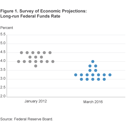
One is that the projections of Federal Open Market Committee members for this rate appear to have fallen. Members announce their forecasts for the long-range nominal federal funds rate, and from them we can infer movements in Committee members’ projections for the real rate by subtracting the long-range inflation objective of 2 percent. In January 2012, the median forecast of Committee members for the funds rate in the longer run was 4.25 percent (figure 1). By March 2016, in the most recently released set of projections, it had fallen to 3.3 percent, a 95 basis point decline. Subtracting the Committee’s inflation objective of 2 percent from each of these forecasts means that the natural interest rate fell from 2.25 percent to 1.3 percent.
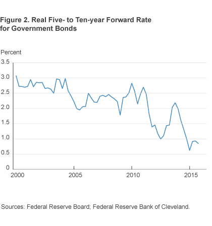
Another way of estimating the natural interest rate is to calculate what markets expect the real short-term interest rate to be on average between five and ten years from now. We use five- and ten-year government bonds to estimate the nominal short-term interest rate in the future, and then we adjust this rate for expected inflation using estimates from a model developed by the Federal Reserve Bank of Cleveland to get the natural rate. This calculation also suggests the natural rate has declined (figure 2). Prior to 2012 this measure of the natural rate averaged more than 2 percent. Recently, however, it has averaged less than 1.5 percent. The decline is nearly basis points.
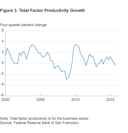
A final indication that the natural interest rate has fallen comes from recent data on productivity growth. Productivity growth is one of the most important determinants of the natural rate, and the data suggest it has declined since the last recession. High productivity growth increases the return on capital investment, leading to a greater demand for investment funds and upward pressure on real interest rates. Lower productivity growth depresses the return to capital and the natural interest rate, all else equal. Before the recession, productivity growth averaged 1.4 percent, but since the start of the recession, it has averaged only 0.4 percent—a full percentage point decline (figure 3).
A Variable Natural Interest Rate in a Taylor Rule
Since the natural interest rate can likely vary over time, we consider how the Taylor rule might be adjusted to capture this variability. We turn to a class of newer macro models in a neo-Wicksellian framework, so-called because they are based on the insights of Kurt Wicksell into interest rates. In these models, the natural rate depends critically on productivity growth. These models suggest that the natural rate will be of the form rt* = r* + αΔzt + 1, where Δzt + 1 is forecasted productivity growth. Recall that productivity growth increases the return to capital investment, putting upward pressure on real rates. But the return is based on future or forecasted productivity growth, so that forecasts drive real rates.
We look at the efficacy of putting such a time-varying natural rate into a standard Taylor rule of the following form:
FRt = r* + 2% + c(rt* − r*) + 1.5(inft − 2%) + 1(GDPt − GDPt*)
If c = 0, this rule is the original rule suggested by Taylor (1999). If c differs from 0, then any change in the natural rate (rt* − r*) will affect the policy prescription for the federal funds rate given by the rule. We assume that productivity growth is measured with error (observed growth = Δzt + met), and that the true value of productivity growth is only observed with a lag. The idea is that the Fed sees a noisy measure of current productivity growth and uses this estimate to forecast future productivity growth and adjust the current funds rate. After one quarter, the true measure of growth is observed, but the Fed cannot change the funds rate it set last quarter.
We consider the effects of different values of c to identify the optimal coefficient on the variable natural interest rate term. The model’s parameters are set to be consistent with standard choices in the literature. We assume that the central bank puts equal weight on the twin goals of minimizing the variability of inflation from a target of 2 percent, and minimizing the gap between output and potential output. We numerically search over possible values of c to determine which value succeeds in minimizing this summed variability.1
If we could perfectly measure productivity growth and thus the natural rate (met = 0), then it is optimal to set c = 1. If the natural rate is measured with error, the preferred size of c is attenuated, that is, less than 1. As we vary the “signal-to-noise ratio” from zero to infinity, c decreases from 1 to 0. But even with substantial noise in the rule (where half of the new information is worthless and half is valid), c is still close to one, c = 0.87.
Measurement Error in Potential Output
The analysis at this point suggests that the optimal response to the measured natural rate of interest be close to one. The attenuation of the response to the natural rate arises only because productivity growth is measured with error. But in the original Taylor rule, the monetary authority also responds to the output gap, which depends on knowing the level of potential output. We therefore must also consider a situation in which both potential output and the natural rate are measured with error.
In the neo-Wicksellian framework, the natural rate of interest is defined to be the hypothetical interest rate that would prevail if there were no stickiness in prices or wages. The theoretical notion of potential output is symmetric: It is the level of output that would prevail without these price and wage rigidities. This implies that if the natural rate is not measured correctly, then neither is potential output. Moreover, these measurement errors are correlated: If potential output is overestimated, then the natural rate is overestimated, and the output gap is underestimated. The fact that the measurement error affects the natural rate and the output gap in opposite ways has important implications for the optimal choice of c because the two measurement errors will often cancel each other out.
We again use a standard macro model to consider the efficacy of different values of c when both the output gap and the natural rate of interest are measured with error. We assume that measurement error accounts for half of the variability in measured productivity growth. Recall that if there were no measurement error, then the optimal choice would be c = 1. But with measurement error there are now two contrasting effects. The first effect is the attenuation effect highlighted earlier: If the natural rate is measured with error, then it is natural to respond less to it so that the optimal c falls below one.
The second effect is that the output gap is measured with error, an error that is negatively correlated with the natural rate measurement error. In this case, two wrongs make a right: A sufficiently large response to the mismeasured natural rate will cancel out the mismeasurement in the output gap. In the extreme, if all movements in measured productivity growth are spurious, then for the parameter values used in our model this second measurement-error effect implies a value of c far above unity, c = 2.5.
When we combine these two contrasting effects of measurement error, the model suggests that the optimal response to the measured natural rate is c = 1.21. This coefficient falls to c = 1.06 if measurement error accounts for only one-fourth of the observed movements in productivity growth. Hence, even with measurement error, there is a strong case for including time-varying estimates of the natural rate in an otherwise standard Taylor rule.
Policy Implications
Simple, Taylor-type policy rules suggest that movements in the natural rate should alter the path of the funds rate only if permanent movements in productivity growth lead to permanent movements in the natural rate. In contrast, the analysis outlined in this article suggests that it may be beneficial for the Fed to include time-varying estimates of the natural rate in its deliberations over the appropriate path of the funds rate, and that these responses are warranted whether these movements are temporary or permanent. More surprisingly, this policy suggestion is reinforced by the possibility of measurement error because this error will affect estimates of the output gap and the natural rate in opposite directions.
We have also presented evidence suggesting that the natural interest rate has declined by as much as 95 basis points. Other things equal, this decline would suggest that the post-liftoff Fed may find it appropriate to raise the funds rate more slowly toward historical levels than if the natural rate had stayed constant.
Footnotes
- We use the standard dynamic new Keynesian model as in Gali (2015) and Woodford (2003). We assume a risk aversion coefficient of unity, a Frisch-labor elasticity of ½, and a personal impatience rate of 2 percent. Firms have a linear labor-only production technology and re-set nominal prices on average every 7 quarters. The central bank policy rule is as in the text. Return to 1
References
- Galí, Jordi, 2015. Monetary Policy, Inflation, and the Business Cycle: An Introduction to the New Keynesian Framework and Its Applications, Second Edition, Princeton University Press.
- Taylor, John B., 1999. “A Historical Analysis of Monetary Policy Rules,” NBER Chapters, in: Monetary Policy Rules, pp. 319-348 National Bureau of Economic Research, Inc.
- Woodford, Michael, 2003. Interest and Prices: Foundations of a Theory of Monetary Policy, Princeton University Press.
Suggested Citation
Carlstrom, Charles T., and Timothy S. Fuerst. 2016. “The Natural Rate of Interest in Taylor Rules.” Federal Reserve Bank of Cleveland, Economic Commentary 2016-01. https://doi.org/10.26509/frbc-ec-201601
This work by Federal Reserve Bank of Cleveland is licensed under Creative Commons Attribution-NonCommercial 4.0 International

