

- Share
On the Relationships between Wages, Prices, and Economic Activity
We take a closer look at the connections between wages, prices, and economic activity. We find that causal relationships between wages and prices are difficult to identify, and the ability of wages to help predict future inflation is limited. Wages appear to be useful in assessing the current state of labor markets, but they are not necessarily sufficient for thinking about where the economy and inflation are going.


The views authors express in Economic Commentary are theirs and not necessarily those of the Federal Reserve Bank of Cleveland or the Board of Governors of the Federal Reserve System. The series editor is Tasia Hane. This paper and its data are subject to revision; please visit clevelandfed.org for updates.
Labor costs and labor compensation have garnered considerable attention from economists in the wake of the financial crisis and recession. Across a range of measures, wage growth slowed sharply during the recession. Recently, wage growth has remained near historically low levels despite improvements in the labor market.
Subdued wage growth has been variously seen as both a cause and a consequence of the slow pace of economic growth and persistently low inflation rates. It also may have contributed to rising inequality. In some forecast narratives, a pickup in wage growth is viewed as a necessary condition for a stronger recovery and rising inflation. In others, it is a natural consequence of a tightening labor market.
This Commentary takes a closer look at the relationships between wages, prices, and economic activity. It finds that the connections among wages, prices, and economic activity are more akin to a tangled web than a straight line. In the United States, wages and prices have tended to move together, and causal relationships are difficult to identify. We do find that wages are sensitive to economic activity and the level of slack in the economy, but our forecasting results suggest that the ability of wages to help predict future inflation is limited. Thus, wages appear to be useful in assessing the current state of labor markets, but not necessarily sufficient for thinking about where the economy and inflation are going.
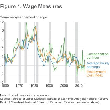
“Wage” Measures
There are a variety of ways to measure labor compensation and labor costs. Our analysis focuses on three such measures. While these measures have varying coverage, we will generically refer to them as “wages.”1
- Average hourly earnings (AHE) of production and nonsupervisory employees on private nonfarm payrolls. This measure is perhaps the closest of our measures to the concept of wages.
- Compensation per hour (CPH) in the nonfarm business sector. This broader measure of compensation includes not only wages but also bonuses and benefits.
- The Employment Cost Index (ECI)—in particular, we use the ECI measuring compensation of private industry workers. The ECI captures wages, salaries, and benefit costs. The ECI abstracts from changes in the sectoral composition of employment over the business cycle, preventing some of the composition bias that affects other wage measures (see Fee and Schweitzer 2011).2
Measures of wage inflation have similar trends, but important differences arise (figure 1). Compensation per hour is notably more volatile than the other wage measures, even when looking at year-over-year growth rates. Abstracting from this volatility, all three wage measures decelerated during the recession, and nominal wage growth has been near 2 percent since the end of the recession—which is quite low by historical standards, and just ahead of inflation during that time. When viewed over a long time span, the upturn in average hourly earnings growth since mid-2012 and the acceleration in the ECI in the second quarter of 2014 are very small.
Cross-Correlations
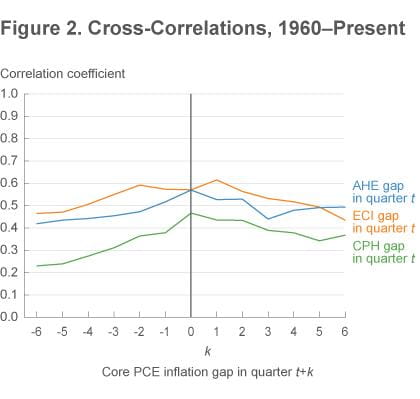
We first consider the connections between wages and inflation or economic activity using cross-correlations. Cross-correlations allow for a simple examination of the lead or lag structure between two series as well as the strength of the connections between the series. If wage inflation reliably comes ahead of price inflation in the data, then the strongest cross-correlation should be between wage inflation in quarter t and price inflation in some k-th quarter after t.
When working with price inflation and wage inflation, there are important long-run trends and short-term volatility that we would like to remove from our analysis. As a general rule, wages and prices have followed roughly similar long-term trends: both accelerated from the 1960s into the 1970s and then decelerated in the 1980s. The forecasting literature has found gains in inflation forecasting accuracy by specifying inflation in gap form as a deviation from a slow-moving long-run trend (see, e.g., Kozicki and Tinsley 2001, Clark 2011, and Zaman 2013). We borrow from this literature and construct wage inflation gaps as quarterly annualized growth in a particular wage measure less a shared long-run trend.3 To remove high-frequency fluctuations in food and energy prices in our measure of price inflation, we define the price inflation gap as quarterly annualized core PCE inflation less the shared long-term trend. We then look at cross-correlations between quarterly price inflation gaps at time t+k and quarterly wage inflation gaps at time t.
Our measures have been moderately positively correlated since 1960: both price inflation and wage inflation tend to be above (or below) trend at the same time (figure 2). The strongest correlations have been between core PCE inflation and the ECI. The weakest correlations have been with the CPH measure, which is not surprising given its volatility. Depending on the measure, wages either lead core PCE inflation very slightly or are contemporaneous with it: the correlation peaks come in quarter t+1 or t.
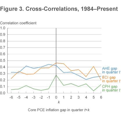
A large literature has identified changes in inflation dynamics since the mid-1980s. If we compute cross-correlations only on the basis of post-1984 data, the results are uniformly weaker (figure 3). The ECI continues to have some of the strongest correlations, especially the contemporaneous relationship between the ECI and core PCE inflation. In this shorter time period, average hourly earnings tend to lag core inflation very slightly: the strongest correlation is between core inflation one quarter in the past (quarter t−1) and AHE inflation today (quarter t).
We can compute similar cross-correlations between a measure of economic activity—for simplicity, we use the Congressional Budget Office’s estimate of the natural rate of unemployment to derive an unemployment gap—and our price and wage inflation gaps. Given that Phillips curves typically relate inflation to economic activity, these cross-correlations are thus one indication of any Phillips curve–like relationships and their timing (figure 4: solid lines show cross-correlations using data from 1960 onward, and dotted lines show cross-correlations using data from 1984 onward). The correlations are negative, consistent with elevated unemployment putting downward pressure on wage and price inflation.
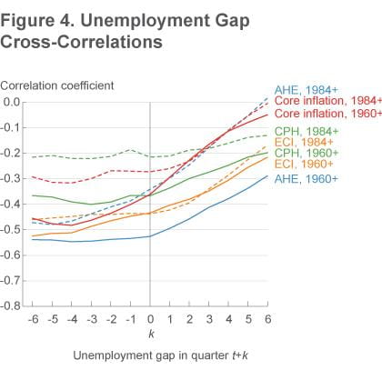
In terms of timing, unemployment gaps tend to lead price and wage inflation gaps: most of the strongest correlations occur when k is negative. For most measures, the correlations are weaker for the post-1984 period, though they are roughly similar for the ECI gaps. Finally, correlations with the unemployment gap are stronger for the ECI gaps than they are for price inflation gaps, potentially suggesting a stronger connection between wages and unemployment than between prices and unemployment—i.e., a stronger wage Phillips curve than a price Phillips curve.
Estimating In-Sample Relationships
While cross-correlations are instructive, they cannot fully capture complicated dynamics. More formally, we use empirical Phillips curves to estimate the in-sample relationships between economic activity and price inflation or wage inflation.4
One of the more robust results we find is that there has not been a stable price Phillips curve since the mid-1980s, but there has continued to be a wage Phillips curve (table 1).5 Over the longer period from 1960 onward, the price Phillips curve respectably fits the data: the unemployment gap is statistically significant, suggesting that price inflation has responded to economic activity as captured by the labor market. Since 1984, however, the price Phillips curve only “fits” the data because of the inclusion of lagged inflation in the empirical model; the unemployment gap is not statistically significant, suggesting little relationship between inflation and slack. By contrast, the unemployment gap has remained statistically significant and economically meaningful in the wage Phillips curve regressions since the mid-1980s.6 These results suggest that subdued wage growth is symptomatic of the existence of slack in the labor market, more so than subdued inflation.
Table 1. Empirical Phillips Curves
| Core PCE inflation gap | ECI inflation gap | AHE inflation gap | CPH inflation gap | |||||
|---|---|---|---|---|---|---|---|---|
| 1960- | 1984- | 1960- | 1984- | 1960- | 1984- | 1960- | 1984- | |
| Constant | 0.09 (0.06) |
−0.15** (0.07) |
0.36*** (0.14) |
0.23** (0.11) |
0.28*** (0.10) |
0.18** (0.08) |
1.29*** (0.31) |
1.30*** 0.93) |
| 1st lag | 0.53*** (0.07) |
0.27*** (0.09) |
0.11* (0.06) |
0.27*** (0.10) |
0.26*** (0.07) |
0.43*** (0.09) |
−0.03 (0.07) |
−0.12 (0.10) |
| 2nd lag | 0.29*** (0.08) |
0.25*** (0.09) |
0.05 (0.06) |
0.24** (0.10) |
0.16** (0.07) |
0.19* (0.10) |
0.14** (0.07) |
0.08 (0.10) |
| 3rd lag | −0.02 (0.08) |
−0.01 (0.09) |
0.19*** (0.06) |
0.11 (0.09) |
0.19*** (0.07) |
0.07 (0.10) |
0.13** (0.07) |
0.04 (0.10) |
| 4th lag | 0.01 (0.07) |
0.09 (0.09) |
0.43*** (0.06) |
0.14 (0.09) |
0.19*** (0.07) |
0.18* (0.09) |
0.18*** (0.07) |
0.08 (0.09) |
| UR gap (t) | −0.13*** (0.04) |
−0.06 (0.04) |
−0.20*** (0.06) |
−0.12** (0.06) |
−0.21*** (0.06) |
−0.12** (0.05) |
−0.52** (0.14) |
−0.48** (0.25) |
| Adj. R2 | 0.66 | 0.26 | 0.54 | 0.52 | 0.65 | 0.75 | 0.19 | 0.03 |
Notes: Stars denote statistical significance at the 10% (*), 5% (**), or 1% (***) level. Standard errors are in parentheses. The unemployment rate gap enters the regressions contemporaneously (at time t).
Of course, Phillips curves suffer from many limitations. There are well-documented instabilities in price Phillips curve relationships (e.g., Stock and Watson 2007), and estimates are extremely sensitive to model specification, variable selection and transformation, sample periods, and a host of other issues. For example, we do not exploit potential asymmetries (e.g., Stock and Watson 2010 for prices; Fee and Schweitzer 2011 for wages) or differences between total unemployment and short-term unemployment in measuring labor market slack (c.f. Gordon 2013).
Further insight into the relationships between wage inflation and price inflation comes from Granger-causality studies. In a nutshell, x is said to “Granger cause” y if past values of x tend to help explain current values of y—but Granger causality need not imply true causality, in which the occurrence of x actually produces the outcome y. The results in this literature are quite mixed but lean slightly toward suggesting that price inflation Granger causes wage inflation (see, e.g., Hess and Schweitzer 2000 for early work). Similar to Phillips curves, however, Granger-causality tests are highly sensitive to issues such as model specification, variable selection, and the sample period under consideration. Hu and Toussaint-Comeau (2010) present a recent survey and find some evidence that prices Granger cause wages between 1960 and 2009, but they find no significant causality since 1984.
Using our three wage measures and core PCE inflation, we extend the Hu and Toussaint-Comeau (2010) findings for several additional years of data. Similar to that study, we also find no evidence of significant Granger causality running in either direction since the mid-1980s, a result that appears to be quite robust.7 These results are consistent with the idea that disentangling wage and price movements is extremely difficult.8
Despite some of these empirical challenges, there are plenty of reasons to believe that connections between economic activity, wages, and prices do exist. The benchmark model for price inflation—the New Keynesian Phillips curve—posits that price inflation today is a function of expected future price inflation and the current marginal costs of production; by iterating forward, price inflation today depends on current and expected future marginal costs (Galí and Gertler 1999, Sbordone 2002). And marginal costs will generally depend on wages, especially in more labor-intensive industries.9 So even if price inflation may empirically appear to Granger-cause wages in some circumstances, current and expected future wages and other components of costs may actually be driving the inflation process in theory.10
Out-of-Sample Forecasting
As a final test, we consider the ability of wage measures to help in predicting future inflation. The previous exercises looked at in-sample relationships and found scant evidence that wages lead prices even within-sample. Out-of-sample forecasting is often a more difficult challenge because relatively weak relationships may change or break down with the passage of time.
Evidence from the forecasting literature that wages and compensation measures help to predict inflation out-of-sample is limited. For example, Stock and Watson (2008) look at inflation forecasts generated using a very wide range of predictors. While they do not exhaust the range of wage measures, the results they present using average hourly earnings to forecast inflation are not very favorable: average hourly earnings provide little help in predicting future inflation compared with a benchmark model in which inflation only depends on its own past readings. The general sensitivity of Phillips curve relationships documented earlier also limits their ability to generate highly accurate out-of-sample forecasts (e.g., Faust and Wright 2013).
We look at the role that wages play in some of the medium-scale macroeconomic models we use to inform forecasting and policy analysis at the Cleveland Fed. The statistical model we present is a Bayesian vector autoregression (BVAR) that includes eight variables: real GDP, real personal consumption expenditures (PCE), core PCE inflation, PCE inflation, productivity, one measure of wages, the unemployment rate, and the federal funds rate.11 The measure of wages, PCE inflation, and core PCE inflation are all modeled in gap form as described earlier. We run three variants of our BVAR including wages—one variant using ECI, one using AHE, and one using CPH—and then run a final variant that excludes any wage measure. The estimation starts in 1959.
To see how well the model forecasts core PCE inflation, we produce quarterly out-of-sample forecasts for the period 1994-2013. We rely on the real-time data that a forecaster would have had available in the middle of each quarter to produce forecasts for the next 12 quarters. For the few series where true real-time data are not available, we used pseudo real-time data instead.12
Our out-of-sample forecast exercises find very slight improvements in inflation forecast accuracy when we include a wage measure compared with the case in which we exclude wages (figure 5). The root mean squared errors (RMSEs)—roughly equivalent to the typical forecasting “miss”—for the forecasts coming from the BVAR without any wage measure are 0.7 percentage point at a four-quarter horizon and 1.0 percentage point at a twelve-quarter horizon. The RMSEs are essentially the same when we include AHE or CPH as the measure of wages (and are therefore difficult to see in the figure), implying that these measures do not help in forecasting core inflation. Using the ECI as the wage measure does reduce the RMSEs, but the differences are trivially small: we generally see a 0.02 to 0.03 percentage point reduction within a three-year forecasting horizon.13
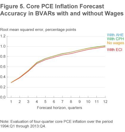
Thus, our forecasting results suggest that the ability of wages to help predict future inflation is limited.
Conclusion
The slow growth of wages during the economic recovery has rekindled interest in the connections between wages, prices, and economic activity. We take a closer look at these issues from a variety of angles. Our analysis finds that wages and prices tend to move together, complicating efforts to disentangle cause and effect. We document evidence of a more stable wage Phillips curve than a price Phillips curve, which is consistent with the idea that subdued wage growth is symptomatic of the existence of slack in the labor market. But given wages’ limited forecasting power, they are but one piece in a larger puzzle about where the economy and inflation are going.
Footnotes
- See Feroli and Silver (2014) for additional details on these and other wage measures. Early results with unit labor costs did not appear promising; hence we omit them from our analysis] Return to 1
- The CPH series is quarterly and begins in 1947. For the monthly AHE series which begins in 1964, we take quarterly averages. To extend the series back to 1959, we splice the data together with average hourly earnings for production and nonsupervisory employees in goods-producing industries. The ECI is quarterly and begins in 1980. For parts of the analysis, we extend the ECI series back in time to 1959 by backcasting this series on CPH. Return to 2
- Our shared long-run trend for both wages and prices is the survey-based long-run (5- to 10-year-ahead) PCE inflation expectations series from the Federal Reserve Board of Governor’s FRB/US econometric model. Return to 3
- We use gaps—price inflation gaps, wage inflation gaps, and the unemployment gap—within the Phillips curve regressions. We rely on a relatively standard empirical Phillips curve framework featuring a constant, the first four lags of the dependent variable, and the contemporaneous unemployment gap as explanatory variables and keep that framework unchanged for each of our price inflation gap or wage inflation gap measures. For this reason, empirical fit could strictly speaking be improved by varying lag length and the timing of the exogenous variables in each regression. Return to 4
- There are an infinite number of potential exercises to run, and we do not pretend to provide the final word on the state of the Phillips curve. In the results we report here, as well as in additional regressions that we do not report, however, we consistently found this pattern in the price and wage Phillips curves. Return to 5
- Galí (2011) motivates and estimates a theoretical forward-looking wage Phillips curve, which he argues is consistent with the ongoing Great Moderation relationship between wages and unemployment. Return to 6
- Over the entire 1960 onward period, we found some evidence of Granger causality running in both directions (wages Granger causing prices and prices Granger causing wages), though we interpret the ECI results with great caution because this measure was constructed prior to 1980. However, these results appeared far less robust than the uniformly negative (i.e., insignificant) findings for the post-1984 period. Return to 7
- As another example of the difficulties in unraveling causality, contemporaneous wage inflation would be a statistically significant explanatory variable if it were added to nearly all our core PCE Phillips curve regressions, and the same is true if we were to add contemporaneous price inflation to our wage Phillips curve regressions. Additionally, within the Bayesian VAR we estimate below, a positive “structural” shock to wages in an impulse-response exercise drives prices higher, and a positive structural shock to prices drives wages higher. Return to 8
- In particular, Knotek and Bednar (2013) and Knotek and Clark (2014) note the strong connection between ECI inflation and core PCE services inflation, including the sharp declines in both inflation rates during the recession; see Peneva (2011) for evidence on the relationship between labor factor intensity and price dynamics. Return to 9
- Empirical support for the canonical New Keynesian Phillips curve is mixed. Matching inflation dynamics usually requires the inclusion of some type of backward-looking behavior, often imposed via ad hoc assumptions (Galí and Gertler 1999; see also Cogley and Sbordone 2008). King and Watson (2012) present one critique. Some recent work within macroeconomic models has pointed to the influences that financial frictions can have on inflation dynamics in an attempt to better match the behavior of inflation following the crisis (e.g., Del Negro and Schorfheide 2013, Gilchrist et al. 2014). Return to 10
- The model is similar to the BVAR in Knotek and Zaman (2013), except that we do not impose the Taylor rule prior on the federal funds rate equation and we split unit labor costs into wages and productivity. Real GDP, real PCE, and productivity enter the model in log levels, while other variables are in levels. Return to 11
- We measure forecast accuracy using the core PCE inflation data available prior to the July 2014 annual revisions. Real-time data come from the Federal Reserve Banks of Philadelphia and St. Louis. Return to 12
- Formal Diebold-Mariano tests cannot reject the null of equal forecast accuracy between the BVAR model without wages and the BVAR model with the ECI at the 5 percent level at any of the forecast horizons shown. We considered several different BVAR specifications that generated roughly similar results to those shown. In some cases, the BVARs with wages reduced RMSEs by 0.1 to 0.2 percentage point; and in some cases, the BVARs with AHE were able to improve upon the forecasting accuracy of the BVAR with ECI. But in the vast majority of cases it was difficult to show statistically that the forecasting accuracy of the models with wages outperformed the models without wages. Return to 13
References
- Clark, Todd E. (2011) “Real-Time Density Forecasts from Bayesian Vector Autoregressions with Stochastic Volatility,” Journal of Business and Economic Statistics, 29(3): 327–41.
- Cogley, Timothy and Argia M. Sbordone (2008) “Trend Inflation, Indexation, and Inflation Persistence in the New Keynesian Phillips Curve,” American Economic Review, 98(5): 2101-2126.
- Del Negro, Marco and Frank Schorfheide (2013) “DSGE Model-Based Forecasting,” in Graham Elliott and Allan Timmermann, eds., Handbook of Economic Forecasting, vol. 2, Elsevier: North Holland.
- Faust, Jon and Jonathan H. Wright (2013) “Forecasting Inflation” in Graham Elliott and Allan Timmermann, eds., Handbook of Economic Forecasting, vol. 2, Elsevier: North Holland.
- Fee, Kyle and Mark E. Schweitzer (2011) “Unemployment, Labor Costs, and Recessions: Implications for the Inflation Outlook,” Federal Reserve Bank of Cleveland, Economic Commentary, 2011-17.
- Feroli, Michael and Daniel Silver (2014) “US: A Field Guide to Wage-Watching,” Economic Research Global Data Watch (July 23, 2014): 1-3.
- Galí, Jordi (2011) “The Return of the Wage Phillips Curve,” Journal of the European Economic Association, 9(3): 436-461.
- Galí, Jordi and Mark Gertler (1999) “Inflation Dynamics: A Structural Econometric Analysis,” Journal of Monetary Economics, 44(2): 195-222.
- Gilchrist, Simon, Raphael Schoenle, Jae Sim, and Egon Zakrajšek (2014) “Inflation Dynamics During the Financial Crisis,” unpublished working paper.
- Gordon, Robert J. (2013) “The Phillips Curve Is Alive and Well: Inflation and the NAIRU During the Slow Recovery,” NBER Working Paper No. 19390.
- Hess, Gregory D. and Mark E. Schweitzer (2000) “Does Wage Inflation Cause Price Inflation?” Federal Reserve Bank of Cleveland, Policy Discussion Paper, no. 1.
- Hu, Luojia and Maude Toussaint-Comeau (2010) “Do Labor Market Activities Help Predict Inflation?” Federal Reserve Bank of Chicago, Economic Perspectives, Q2: 52-63.
- King, Robert G. and Mark W. Watson (2012) “Inflation and Unit Labor Cost,” Journal of Money, Credit and Banking, 44(S2): 111-149.
- Knotek, Edward S. II, and Saeed Zaman (2013) “When Might the Federal Funds Rate Lift Off? Computing the Probabilities of Crossing Unemployment and Inflation Thresholds (and Floors),” Federal Reserve Bank of Cleveland, Economic Commentary, 2013-19.
- Knotek, Edward S., II and Todd E. Clark (2014) “Inflation: Why It Is Very Low, and Why It Matters,” Federal Reserve Bank of Cleveland, Annual Report 2013.
- Knotek, Edward S., II and William Bednar (2013) “Behind Recent Disinflation: 2010 Redux?” Federal Reserve Bank of Cleveland, Economic Trends, 06.24.2013.
- Kozicki, Sharon and P.A. Tinsley (2001) “Shifting Endpoints in the Term Structure of Interest Rates,” Journal of Monetary Economics, 47(3): 613-52.
- Peneva, Ekaterina (2011) “Some Evidence on Factor Intensity and Price Rigidity,” Journal of Economic Dynamics and Control, 35(10): 1652-58.
- Sbordone, Argia M. (2002) “Prices and Unit Labor Costs: A New Test of Price Stickiness,” Journal of Monetary Economics, 49(2): 265-292.
- Stock, James H. and Mark W. Watson (2007) “Why Has U.S. Inflation Become Harder to Forecast?” Journal of Money, Credit and Banking, 39(S1): 3-33.
- Stock, James H. and Mark W. Watson (2008) “Phillips Curve Inflation Forecasts,” NBER Working Paper No. 14322.
- Stock, James H. and Mark W. Watson (2010) “Modeling Inflation after the Crisis,” in Macroeconomic Challenges: The Decade Ahead—A Symposium Sponsored by the Federal Reserve Bank of Kansas City, Federal Reserve Bank of Kansas City: Kansas City, MO.
- Zaman, Saeed (2013). “Improving Inflation Forecasts in the Medium to Long Term,” Federal Reserve Bank of Cleveland, Economic Commentary, 2013-16.
Suggested Citation
Knotek, Edward S., II, and Saeed Zaman. 2014. “On the Relationships between Wages, Prices, and Economic Activity.” Federal Reserve Bank of Cleveland, Economic Commentary 2014-14. https://doi.org/10.26509/frbc-ec-201414
This work by Federal Reserve Bank of Cleveland is licensed under Creative Commons Attribution-NonCommercial 4.0 International

