The Slowdown in Residential Investment and Future Prospects

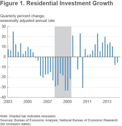
Housing has historically been a key driver of the U.S. economy. Many past recessions have either coincided with or been caused by downturns in the housing market, and turnarounds in residential investment have helped propel past economic recoveries.

Today, the housing market has improved markedly compared with where it was during the depths of the financial crisis. But concerns linger over the state of residential investment, and activity generally remains at low levels. Contributing to the concern is the fact that residential investment contracted in the past two quarters—the first consecutive quarterly declines since the end of the recession (figure 1).

We disentangle the causes of the recent slowdown in residential investment using a statistical model, and we examine the future prospects for this important sector of the economy. Our model points to three primary factors behind the recent weakness: the increase in mortgage rates since early 2013, the unusually cold winter, and a modest tightening of lending standards in the residential mortgage market. The model suggests that with normal weather and ongoing improvements in labor markets and the broader economy, growth in residential investment should rebound soon. But the experiences of the past year highlight the key role of mortgage rates and the strong interest rate sensitivity of the housing sector. Our forecasts suggest that even moderate increases in mortgage rates through the end of next year could pose a headwind to residential investment. Put differently, mortgage rates that remain low by historical standards are likely to be an important factor underlying ongoing recovery in the housing market and, by extension, the economy overall.

A Model of Residential Investment

To empirically capture the relationship between residential investment and its key determinants, we use a statistical model known as a Bayesian vector autoregression (BVAR). Our model includes variables that are significant for the U.S. economy and that are expected to have a strong influence on residential investment. Our medium-scale BVAR model includes eleven variables, in the following order: a measure of weather conditions (defined below), real gross domestic product (GDP), real personal consumption expenditures (PCE), a measure of lending standards, a survey-based indicator of consumers’ perceptions of home-buying conditions, real residential investment, the unemployment rate, core PCE inflation, PCE inflation, CoreLogic home prices, and the 30-year mortgage rate.¹

A few variables merit explanation. Our weather measure captures unseasonably cold temperatures: a large positive weather reading, as occurred in 2014:Q1, is consistent with colder-than-usual temperatures.² To capture lending standards, we look to the Federal Reserve Board’s Senior Loan Officer Opinion Survey on Bank Lending Practices (SLOOS) and use the net percentage of domestic respondents who report tightening standards for residential mortgages.³ Having been negative through mid-2013, SLOOS-based readings have been positive for the last two quarters, and positive readings indicate a net tightening of lending standards. Finally, consumers’ perceptions of home-buying conditions are measured by a diffusion index that subtracts the percentage of consumers reporting that it is a bad time to buy a home from the percentage reporting that it is a good time to buy a home in the Thomson Reuters/University of Michigan Survey of Consumers.

Decomposing the Recent Past

While our model is relatively simple, it can effectively explain the recent weakness in residential investment. Formally, we employ a decomposition to see what the model would have predicted at some previous point in time and then identify what caused the data to diverge from that forecast.⁴ To do so, we estimate the model using quarterly data from 1990:Q4 through 2012:Q4 and then generate a forecast for residential investment growth through 2014:Q1.

This baseline forecast calls for residential investment activity to have remained strong through 2014:Q1 (figure 2). And through 2013:Q3, the baseline forecast tracked the actual path of residential investment well. But residential investment growth fell off sharply in the data in 2013:Q4, and activity contracted again in 2014:Q1. The decline was so sudden and large that the data are near the lower 90 percent confidence band around the forecast, which puts them in the very bottom tail of the distribution of outcomes that the model would characterize as reflecting normal historical uncertainty. What happened?

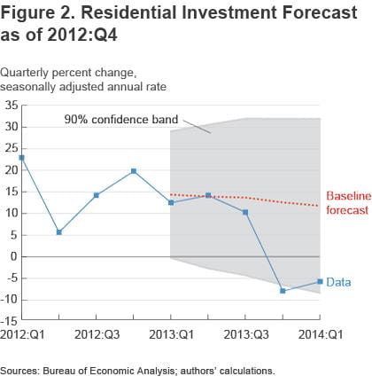
To answer this question, we look at forecast errors, which are the differences between the baseline forecast and the actual data. For example, in 2013:Q4, the forecast called for residential investment to grow 13 percent, while the actual reading was −8 percent, for a forecast error of 21 percentage points. The forecast error in 2014:Q1 was almost as large.

Our BVAR allows us to decompose these historical forecast errors by examining the unanticipated events, or shocks, that drove our model variables—in essence, allowing us to compare whether the model is able to explain deviations from the baseline forecast after the fact.⁵ If feeding in a given set of shocks helps to push the model’s forecast toward the actual outcome, then those shocks help explain why the forecast was wrong. We first isolate the shocks that occurred to three key variables—mortgage rates, weather, and lending standards—individually and examine how the forecast changes if those shocks had been known in advance (figure 3).

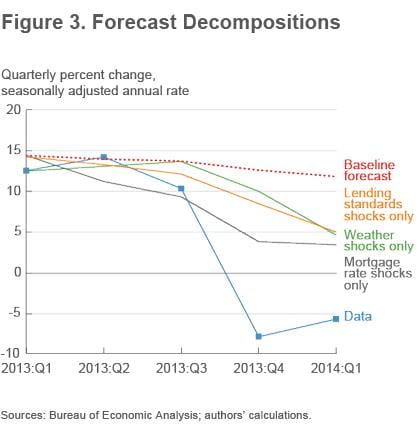
The decomposition suggests that these three variables played major roles in the slowdown of residential investment. For one, the increase in mortgage rates was unanticipated in the baseline forecast. Once we feed in the shocks that drove mortgage rates higher, the path for residential investment is notably weaker and much closer to the actual path that residential investment growth followed. In fact, higher mortgage rates alone explain almost half of the forecast errors in 2013:Q4 and 2014:Q1.

Similarly, the baseline did not anticipate the unusually cold winter weather. Running a second simulation that includes our estimated weather shocks reveals that the weather played a substantial part in restraining residential investment activity in 2014:Q1. Approximately 41 percent of the forecast error in that quarter came from the weather.

The forecast decomposition also reveals that the unexpected tightening in SLOOS-based lending standards over the last two quarters had a restraining effect on residential investment. On average, 30 percent of the forecast errors over those quarters came from the shocks that caused tightening lending standards. (Note that other factors made unexpected positive contributions to residential investment, which explains why these three factors account for more than 100 percent of the forecast errors.)

Finally, we can put together all the estimated shocks (except residential investment’s own shock) and run another simulation to see if we can explain the recent declines in residential investment. Once we account for the shocks to mortgage rates, weather, lending standards, and all our other explanatory variables at the same time, our model explains the past fairly well: it predicts that residential investment should have contracted in both 2013:Q4 and 2014:Q1 (figure 4).

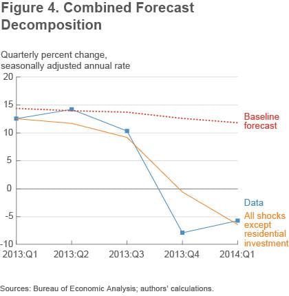
Of course, most of these declines came from high mortgage rates, cold weather, and tighter lending standards. The difference between this simulation and the actual data reflects additional forecast errors; they represent the portion of the data that the model is unable to explain even after the fact and are considered direct shocks to residential investment. The relatively small size of the unexplained forecast errors implies that residential investment followed a different path from the baseline forecast primarily because the main determinants of residential investment moved in unexpected ways.

Residential Investment Going Forward

Our decomposition exercise was fairly successful in identifying key factors behind the recent weakness in residential investment after the fact. By contrast, the baseline forecast had large misses. Thus, this analysis illustrates the dangers inherent in forecasting: unanticipated events can push actual outcomes far from what was expected. So instead of considering a single forecast to anticipate where residential investment may be headed, we consider several scenarios that focus on how these key factors may play out and what each implies for residential investment.

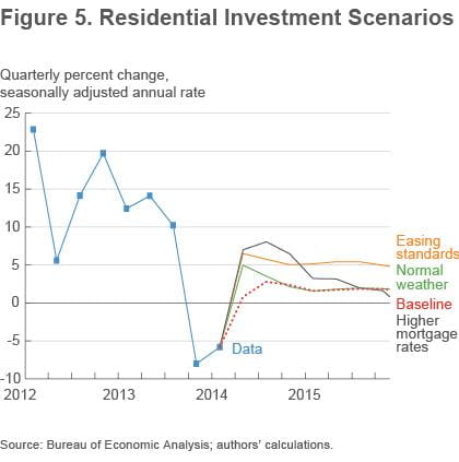
To do so, we first reestimate the model using data through 2014:Q1 and make a baseline forecast for all the model’s variables. This baseline forecast largely extrapolates the recent past into the future (figure 5). As a result, GDP growth recovers slowly, mortgage lending standards remain relatively tight, and the path for residential investment going forward would be quite subdued.

However, there are compelling reasons to believe that the severe winter weather had a temporary impact on the housing sector—after all, winter cannot last forever—and our model allows us to isolate the effects of a return to more normal temperatures. In our first scenario, we assume that temperatures quickly return to normal.⁶ This is known as a conditional forecast, because future outcomes for the other variables in our model, especially residential investment, depend on a specific path or “condition” for a particular variable—in this case, the weather. We also assume that a good portion of the first quarter’s GDP reading can be explained by severe weather and other transitory factors, and we pencil in a second condition that GDP growth rebounds to 3 percent in the second quarter. These assumptions alone generate a sharp recovery in residential investment, as growth quickly turns positive. But the model predicts that the surge would be short-lived, and residential investment growth would decline back to the baseline in a few quarters.

If we peer under the hood of this forecast, the model has mortgage lending standards still remaining tight—in fact, our measure remains positive through the end of 2015. Because the SLOOS-based measure is a diffusion index, positive readings actually imply an ongoing tightening of standards on residential mortgage loans. It is unclear what might drive such an ongoing tightening of standards. Changes in regulations related to qualified mortgages likely explain at least part of the recent tightening, and further changes are uncertain.

Our second scenario assumes that, in addition to the weather assumptions above, this tightening reverses course, and mortgage lending standards ease modestly until the SLOOS measure returns to where it had been at the end of 2013.⁷ This easing of lending standards gives a boost to the housing sector. In this case, residential investment grows at about a 6 percent pace through the end of 2015. The stronger outlook for residential investment helps to promote a virtuous circle in the economy: GDP growth in this second scenario remains near 3 percent through the end of 2015, which in turn provides further support to the housing sector, whereas GDP growth in the first scenario quickly fell back to 2½ percent.

Interest Rate Sensitivity and Residential Investment

In the model we have estimated, there is an important asymmetry. The mortgage rate is not very sensitive to economic conditions, but economic conditions are sensitive to the mortgage rate. A strengthening economy—as occurred in the mid-2000s, for example—has little effect on mortgage rates. In addition, the mortgage rate is difficult to predict, as idiosyncratic shocks are its primary driver. As a result, mortgage rates in the above scenarios are forecasted to end 2015 near their current levels.

Yet the economy is clearly sensitive to mortgage rates. Our earlier decomposition revealed that increases in mortgage rates played the single largest role in the recent weakness in residential investment. The previous projections for residential investment are importantly influenced by stable mortgage rates. Thus, it is worthwhile exploring a scenario in which mortgage rates follow an alternative path.

A flat path for future mortgage rates contradicts economists’ expectations for long-term interest rates going forward. For example, the consensus forecast in the Blue Chip Economic Indicators survey from May 2014 is that 10-year Treasury yields will increase just over 1 percentage point over the next year and a half, from 2.8 percent in the second quarter of 2014 to 3.9 percent in the fourth quarter of 2015. Assuming that the spread between mortgage rates and 10-year Treasury rates remains unchanged, our third scenario builds on the first two by setting mortgage rates on a similar increasing path.⁸

Higher mortgage rates have two effects within our model. In conditional forecasting exercises, higher interest rates initially tend to raise GDP growth, and this stronger GDP growth spills over to boost residential investment growth as well. Our third scenario displays this same pattern. Statistically speaking, this pattern reflects long-term correlations rather than causal relationships: during good times, GDP growth and interest rates are usually high; during bad times, both GDP growth and interest rates are low.

Over time, however, our conditional forecasts show that higher mortgage rates eventually slow the housing market. Quantitatively, the slowing from higher mortgage rates is greater than the boost from easing lending standards in this third scenario. As a result, our model posits that moderate increases in mortgage rates through the end of next year—to a level around 5½ percent, which remains low by historical standards—potentially would pose a headwind to residential investment. And as might be expected, these higher interest rates and slower housing activity eventually weigh on GDP growth in our model as well. This analysis therefore suggests that low mortgage rates are likely to be an important factor underlying ongoing recovery in the housing market and, by extension, the economy overall.⁹

Conclusion

Using a statistical model, we find that three primary factors can explain most of the declines in residential investment at the end of 2013 and the beginning of 2014: the increase in mortgage rates since early 2013, the unusually cold winter, and a modest tightening of lending standards in the residential mortgage market.

Our analysis suggests that the resumption of more normal weather will allow for an imminent rebound in residential investment, and a gradual easing of lending standards stands to lift the outlook for the housing sector going forward. But the experiences of the past year highlight the strong interest rate sensitivity of this sector. Our model forecasts suggest that moderate increases in mortgage rates through the end of next year—to levels that would still be relatively low by historical standards—potentially would pose a headwind to residential investment. Put differently, low mortgage rates are likely to be an important factor underlying ongoing recovery in the housing market and, by extension, the broader economy.

References

- Clark, Todd E., and Saeed Zaman, 2013. “e,” Federal Reserve Bank of Cleveland, Economic Commentary, 2013-15.
- Koop, Gary M., 2013. “Forecasting with Medium and Large Bayesian VARs,” Journal of Applied Econometrics 28(2): 177-203.
- Kozicki, Sharon, and Peter A. Tinsley, 2001. “Term Structure Views of Monetary Policy under Alternative Models of Agent Expectations,” Journal of Economic Dynamics and Control 25: 14-84.
Suggested Citation
Knotek, Edward S., II, and Saeed Zaman. 2014. “The Slowdown in Residential Investment and Future Prospects.” Federal Reserve Bank of Cleveland, Economic Commentary 2014-10. https://doi.org/10.26509/frbc-ec-201410
This work by Federal Reserve Bank of Cleveland is licensed under Creative Commons Attribution-NonCommercial 4.0 International