The State of States’ Unemployment in the Fourth District

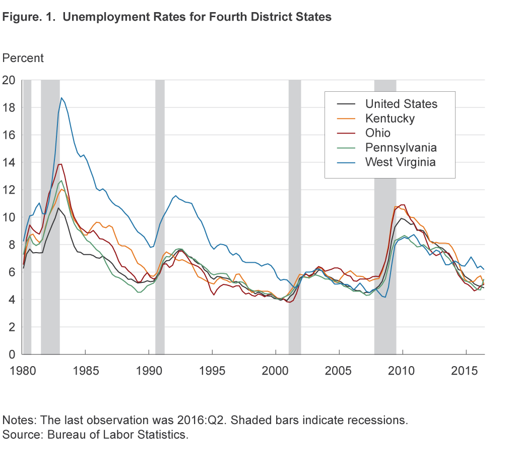
In the last quarter of 2007, on the brink of the Great Recession, the unemployment rate varied by just 1 percentage point across the four states of the Federal Reserve’s Fourth District—Kentucky, Ohio, Pennsylvania, and West Virginia—ranging from 4.7 percent in Pennsylvania to 5.7 percent in Ohio.¹ As the US economy entered the recession, unemployment rates increased sharply in all four states, but the magnitude of the increases differed dramatically across them. The two states with higher unemployment rates prior to the recession, Kentucky and Ohio, saw much greater increases (5.3 percentage points and 5.2 percentage points, respectively) than did Pennsylvania and West Virginia (4.0 percentage points and 3.7 percentage points, respectively), both of which started from relatively lower levels. In previous decades, the variation in the unemployment rates across states was typically much larger (figure 1).

In this Economic Commentary, we put these states’ unemployment numbers into context. We describe the “normal” unemployment rate for each of the four states and compare it to the national normal. Then we calculate how far the current unemployment rates in the District are from normal. Because the difference between the current and normal rates usually indicates underutilized resources in the labor market, or “labor market slack,” it is an important issue for policymakers.

A Trend Concept for State Unemployment

To gauge the normal level of the unemployment rate at the state level, we follow the methodology of Tasci (2012). That methodology aims to find an estimate for the long-run trend of the national unemployment rate using data on worker flows into and out of unemployment.

Tasci’s main premise is that the unemployment rate at a point in time as a stock variable is determined by two opposing flows: inflows from employment into unemployment (“EU”) and outflows from unemployment to employment (“UE”). The long-run trend levels of these underlying flows determine an implied trend for the unemployment rate. This implied trend can be understood as the unemployment rate that is attainable in the long run, when the cyclical variations in the underlying EU and UE flows disappear and the labor market functions normally.

A key challenge involved in this approach is separating the trend component from the business cycle in the observed flows. The EU flow rate, for instance, is significantly countercyclical, implying higher rates of separation from existing jobs in downturns. The UE flow rate, on the other hand, is strongly procyclical and quite volatile. These cyclical changes in the flow rates cause the fluctuations in the unemployment rate over the business cycle. Tasci tackles the problem of separating the trend component from these cyclical fluctuations by estimating the underlying trends in EU and UE flows with a statistical model. The model identifies the trend components of the data on EU and UE flows by removing the cyclical components, which are treated as dependent on business-cycle movements in output.

Once we have the implied (unobserved) trends in the EU and UE flow rates, the trend unemployment rate is easily calculated from a simple relationship: u* = EU*/(EU*+UE*), where u*, EU*, and UE* are the trend rates in unemployment, EU, and UE, respectively. The easiest way to understand this relationship is via a bathtub analogy: One can think of the level of the water in a bathtub at any point in time like the stock of unemployment. As long as the flow of water into the tub (EU) is greater than the flow of water draining out (UE), water in the tub will continue to rise. Only when these flows offset each other will the water stay level. Similarly, when the flow rates are at EU* and UE*, the unemployment rate stays constant at u*. Therefore, the unemployment trend in the long run is related to the underlying trends of the flow rates at a fundamental level.

In order to adapt the methodology from Tasci’s analysis of the nation to the analysis of Fourth District states, we have to consider two other transitions that take place in the labor market. One is the transition to and from nonparticipation in the labor force. Not all transitions into unemployment come from employment, and some transitions into employment are due to movements of people who were not previously unemployed. A new college graduate starting to look for a job or a retired worker who takes a part-time job after being out of the workforce for several years are two examples of such transitions. Tasci shows that the estimated unemployment rate trend, u*, for the nation is unaffected when this transition is included, but it is not clear whether this would be true for all states in the nation. For instance, if some states have a larger group of workers around retirement age, flows from employment to nonparticipation might take a more prominent role for those states. This possibility requires us to allow for more flexibility in the model to include transitions between nonparticipation (N) and employment (E) or unemployment (U).

Similarly, movements of workers between states because of interstate migration could prove to be an important determinant of the changes in the unemployment stock and the labor force within a state over time. This movement is irrelevant for the national data, as the migration flows in and out of the nation are too small to have a material effect on u*. However, we cannot rule out the importance of this channel for some states. For instance, we know there has been a gradual population shift from northern states to southern states. In addition, southern states had disproportionately larger flows of immigrant workers into the states from outside the nation. Hence, we need to modify Tasci’s approach to allow for these additional flow rates at the state level.

Unfortunately, capturing the true extent of the last two flow rates for the states in the Fourth District, let alone for every state in the nation, is not feasible. Interstate migration is notoriously ill-measured, and for many of the small states, flows involving the nonparticipation margin come from very small samples of surveyed respondents, making measures of nonparticipation imprecise. In addition to these measurement issues, incorporating all four different labor market statuses and the bilateral flows among them would require modeling 12 different transition rates. These additional flow rates impose high computational costs, and the model becomes intractable quickly. Instead, we adopt a simpler strategy to tackle this problem by essentially collapsing two different statuses (nonparticipation and out-of-state migration) into one, “Q.” We follow this simplification to obtain the estimates for the unemployment trend for the states within the Fourth District.

As a result of this simplification, we keep track of the movements in four different flows. Two of them are the usual flows that Tasci focused on as well, EU and UE. The remaining two flows are the transitions that involve Q. One of these transitions ends up increasing the unemployment stock on net, and we refer to it as “nQU.” Similarly, the net flows involving Q that increase the employment stock, on net, will be called, “nQE.” Hence, we have an extended model of Tasci’s with additional flow rates that might be important at the state level. Once we obtain the unobserved trend estimates for all four flow rates, the state-level unemployment trend is defined by u* = (EU* + nQU*)/(EU* + nQU* + UE* + nQE*). As in the simpler case we discussed above, when flow rates are at their corresponding starred (*) levels, the unemployment rate stays at its trend level, u*.

In this implementation of Tasci’s model, identifying the cyclical components of the flow rates at the state level requires us to find a measure of state-level economic activity at a relatively high frequency. For this purpose, we use the Federal Reserve Bank of Philadelphia’s quarterly coincident activity index at the state level, going back to 1979. Thus, we can reliably estimate the unemployment trends for the states in the Fourth District from 1979 through 2016.

Converging Trends, Disappearing Slack

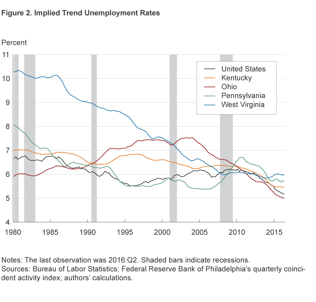
Figure 2 shows our estimates for the unemployment rate trends for all the states in the Fourth District along with the aggregate trend estimated for the nation. Estimated trends display a great deal of dispersion early in the sample, ranging from 6 percent for Ohio to more than 10 percent for West Virginia. For most of the first two decades of the sample, the estimated trend for West Virginia stayed well above the trend level estimated for the other states in the Fourth District and for the nation as a whole. By the end of the sample period, the trend estimates settled within a narrow band, from 5 percent to 6 percent. For example, as of the second quarter of 2016, the estimated trend rate of unemployment for Ohio is 5.0 percent. Corresponding numbers for Kentucky, Pennsylvania, and West Virginia are 5.5 percent, 5.7 percent, and 6.0 percent, respectively. The national trend stood at 5.2 percent then. Note also that by the second quarter of 2016, the range of trend unemployment rate estimates is very similar to the range of actual unemployment rates for each of the Fourth District states and the nation.

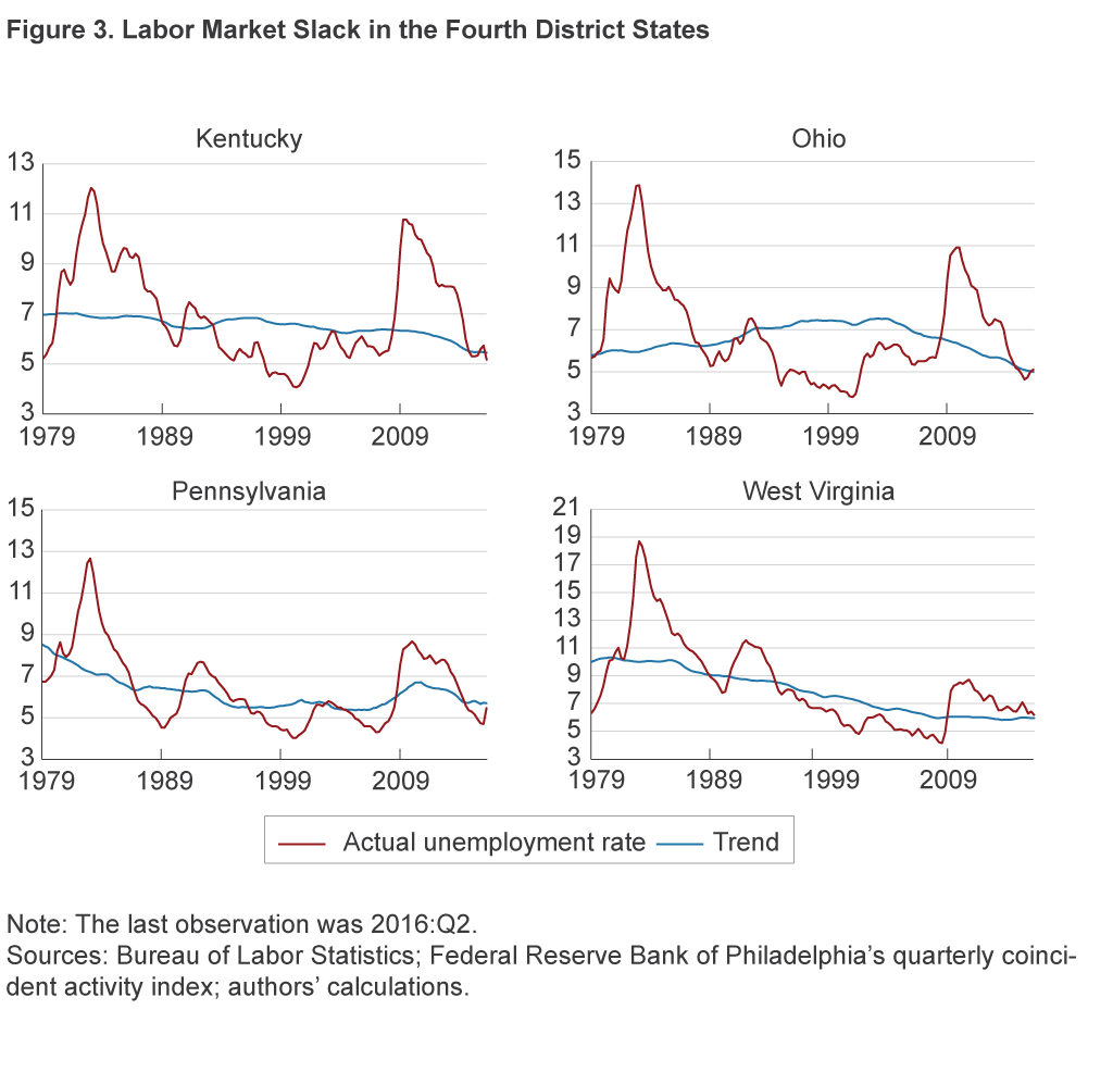
The proximity of the observed level of unemployment to the estimated trend indicates that the labor market has removed most of the cyclical slack that appeared during the recession (figure 3). That is to say, almost seven years after the Great Recession came to an end, labor markets at the state level within the Fourth District finally have reached a rate of unemployment that is consistent with normal turnover. These estimates and the data indicate that there are not as many underutilized resources in the labor market as there were throughout the recession.

As noted above, the Federal Reserve’s Fourth District consists of the entire state of Ohio but only parts of Pennsylvania, Kentucky, and West Virginia. So far we have used estimated trends and rates with data for the entirety of each state within the District. To calculate a District unemployment rate and a District trend, we therefore need to adjust the rates we have estimated for the states. We create a representative District labor market by weighting the observations at the state level by the share of the labor force in those states that works in the Fourth District.

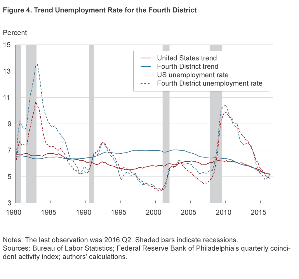
Figure 4 compares the state of the labor market in the District to the national situation. We see that the District unemployment rate is basically at the trend level we estimated. Similarly, the national labor market is close to the trend we estimated. In fact, if we define labor market slack as the difference between the estimated trend and the observed level of unemployment, we observe that labor market slack in the Fourth District since the Great Recession seems to have moved in tandem with that of the aggregate economy. This correspondence stands in contrast to the rest of the sample period. First, early in the 1980s, despite similar estimated trends, District unemployment was much higher, indicating more slack in the region. This observation is consistent with the major hit the manufacturing sector experienced during the downturns in the 1980s. Because they had a larger share of employment in the manufacturing sector, states in the Fourth District were disproportionately affected by the downturns. Starting with the 1990s, however, the estimated trends diverged substantially, despite similar movements in the unemployment rate. This divergence indicates that, compared to the national labor market, District labor markets were relatively tighter for most of the 1990s until the Great Recession.

Conclusion

In light of large unemployment fluctuations following severe business-cycle episodes such as the Great Recession, evaluating what constitutes a normal level for the unemployment rate at the state level is an important issue for policymakers. In this Economic Commentary, we introduce a framework to gauge where the labor market stands in each state of the Fourth District in terms of the unemployment rate statistic. We conclude that individual states in the District (as well as the District as a whole) have almost no labor market slack remaining as of the end of the second quarter of 2016. By this metric, local labor markets do not seem to be any different than the aggregate national labor market.

References

- Tasci, Murat, 2012. “The Ins and Outs of Unemployment in the Long Run: Unemployment Flows and the Natural Rate,” Federal Reserve Bank of Cleveland, Working Paper no. 12-24.
Suggested Citation
Tasci, Murat, Caitlin Treanor, and Christopher Vecchio. 2017. “The State of States’ Unemployment in the Fourth District.” Federal Reserve Bank of Cleveland, Economic Commentary 2017-02. https://doi.org/10.26509/frbc-ec-201702
This work by Federal Reserve Bank of Cleveland is licensed under Creative Commons Attribution-NonCommercial 4.0 International