

- Share
Measuring Inflation Forecast Uncertainty
Looking across a range of statistical models, we consider the likely path of future inflation and the uncertainty surrounding the models’ predictions. The models suggest that inflation is on a rising path, and while inflation forecast uncertainty is somewhat elevated relative to the norms of the last 20 years, core inflation uncertainty is relatively low. For both inflation rates, forecast uncertainty is much lower as of the first quarter of 2015 than it was around the Great Recession.


The views authors express in Economic Commentary are theirs and not necessarily those of the Federal Reserve Bank of Cleveland or the Board of Governors of the Federal Reserve System. The series editor is Tasia Hane. This paper and its data are subject to revision; please visit clevelandfed.org for updates.
The federal funds target range has been zero to one-quarter percent since late 2008. But a number of signs suggest that change may be drawing near. In their projections made for the March 2015 meeting, all but two Federal Open Market Committee (FOMC) participants believed that it would be appropriate to increase the federal funds rate target range in 2015. In their post-meeting statement, the Committee anticipated that “it will be appropriate to raise the target range for the federal funds rate when it has seen further improvement in the labor market and is reasonably confident that inflation will move back to its 2 percent objective over the medium term.”1
With ongoing solid readings coming from the labor market, this Commentary examines the outlook for inflation. Looking across a range of statistical models, we consider where inflation is likely to go in the future. In doing so, we look at not only the most likely future path for inflation but also the uncertainty around that path—that is, how confident the models are about their own predictions.
Our models generally put inflation on a rising path: inflation in two years is expected to be greater than inflation in one year. In an absolute sense, the uncertainty surrounding these projections is large, but this comes as no surprise—it is well known that forecasting inflation far into the future is always difficult.2 When we measure how uncertainty today compares with its past values, we find that inflation forecast uncertainty today is perhaps somewhat elevated compared with the norms of the last 20 years, while forecast uncertainty for core inflation is relatively low compared with the same period. But if we focus on the recent past, inflation forecast uncertainty as of the first quarter of 2015 is much lower than it was around the Great Recession, having fallen by two-thirds in some cases.
A Range of Models
Because forecasting inflation is a difficult task, no single model has emerged as “the best” forecasting tool. The simplest inflation forecasting model predicts that future inflation will be equal to its value over the past year; at the other extreme, factor models can combine hundreds of indicators to predict future inflation rates.3 We do not attempt to examine every possible inflation forecasting model. Instead, we present results from five fairly sophisticated statistical forecasting models with good inflation forecasting properties. All of the models use data at a quarterly frequency.
First, we include a relatively standard statistical model used for macroeconomic forecasting and policy analysis: a Bayesian vector autoregression (BVAR). The model follows Knotek and Zaman (2013) and includes seven variables: real GDP, real personal consumption expenditures (PCE), the unemployment rate, unit labor cost growth, PCE inflation, core PCE inflation, and the federal funds rate.4 We estimate this BVAR model using long time series data, starting in 1959:Q1.
Second, we examine the forecasts coming from a medium-scale vector autoregression estimated using Bayesian methods and a steady-state prior (SS-BVAR), in the spirit of Villani (2009). A key benefit of the SS-BVAR is that it allows us to incorporate additional information, potentially coming from outside the model, to inform the model’s longer-run properties; but incorporating this additional information can help with shorter-term forecasting as well. To the list of variables above, we add one more labor market variable (nonfarm payroll growth) and two financial variables (the S&P 500 and the risk spread between Baa corporate bond yields and 10-year Treasury yields).5 We estimate this SS-BVAR model using time series data starting in 1985:Q1, to account for changes in inflation dynamics that occurred around that time.6
Models three through five feature stochastic volatility. In most macroeconomic models, including the two listed above, the size of realized shocks can vary over time, but the shocks are assumed to be drawn from a distribution with a standard deviation that is fixed. Models with stochastic volatility allow the standard deviation of the size of the shocks to change over time. Intuitively, stochastic volatility allows models to rapidly capture the changing size of the shocks hitting the economy. Including this feature in models has been found to improve the historical accuracy of the uncertainty surrounding forecasts. In any event, we estimate all three of these models using the full history of available data, back to 1959:Q1.
Our third model is the unobserved components model with stochastic volatility (UC-SV) of Stock and Watson (2007). The UC-SV model posits that inflation fluctuates around an unobserved trend and is subject to temporary movements away from that trend. The unobserved trend follows a random walk, changing over time only in response to shocks. In addition, the standard deviation of the size of the shocks that move the unobserved trend and the standard deviation of the size of the shocks that generate temporary departures from the trend can both vary over time.8 We label these 2015:Q1 forecasts, to line up with the date at which the forecasts are made. The 2015:Q1 forecasts for PCE inflation and core PCE inflation from each model are in Table 1. In these forecasts, all inflation rates measure inflation over the previous four quarters.
Table 1. Inflation Forecasts as of 2015:Q1
| PCE inflation | ||
|---|---|---|
| 4 quarters ahead | 8 quarters ahead | |
| BVAR | 1.5 | 2.2 |
| SS-BVAR | 2.0 | 2.4 |
| UC-SV | 1.2 | 1.2 |
| SS-SV | 1.1 | 1.7 |
| TVP-SV | 1.2 | 1.5 |
| Core PCE inflation | ||
| 4 quarters ahead | 8 quarters ahead | |
| BVAR | 1.4 | 1.9 |
| SS-BVAR | 1.9 | 2.1 |
| UC-SV | 1.4 | 1.4 |
| SS-SV | 1.2 | 1.5 |
| TVP-SV | 1.7 | 1.8 |
Notes: All numbers show four-quarter inflation rates. Forecasts use data through 2014:Q4.
The consistent message across models is that inflation is likely to rise going forward. In four of the five models, the point forecasts call for inflation to pick up over time: inflation eight quarters in the future is expected to be greater than inflation four quarters in the future. This pattern is true for both PCE inflation and core PCE inflation. As one might expect, different forecasting models have different properties and will produce different forecasts, and that is certainly the case with our exercise. Eight quarters ahead, two forecasts (from the BVAR and SS-BVAR models) predict PCE inflation will be between 2 and 2½ percent, while two forecasts (from the SS-SV and TVP-SV models) predict PCE inflation will be between 1½ and 2 percent.
The one exception to the above is the UC-SV model. In this model, the single best forecast for where inflation will be in the future is entirely dependent on the current estimate of the unobserved inflation trend. Hence, this model generates a perfectly flat forecast path for inflation, even arbitrarily far into the future.
Illustrating Forecast Uncertainty
In general, the uncertainty around the outlook for inflation has two broad sources. First, we face uncertainty about the “true” model of inflation. We have included in this study a number of models, differing along a variety of dimensions, such as: whether inflation is determined by anything other than its own past, what other variables help to determine inflation, and the time period over which the model is estimated. This type of uncertainty can be captured by the dispersion of these forecasts: if some forecasts are rising while others are falling, it indicates considerable uncertainty about the outlook.9 We do not really see this in our current forecasts. All inflation forecasts are rising except for one.
Second, even given a particular model, the inflation forecast is uncertain because we do not know what will happen over the forecast horizon: there will be shocks we cannot anticipate at the time we make the forecast.10 While we have focused on point forecasts so far, we can use each of our models to quantify the uncertainty around the forecast based on the sizes of shocks captured by the model. In particular, the model can also produce the probability that a given event will occur, or the likelihood that the future will evolve within some certain range.11
We illustrate this concept with the BVAR model. Figure 1 shows how this model expects inflation to behave over the next three years, based on the forecast made in 2015:Q1. The solid lines depict the point forecasts. The dashed lines show the 70 percent confidence bands for PCE inflation and core PCE inflation. The confidence bands indicate that the model expects inflation outcomes to fall within this region 70 percent of the time.12
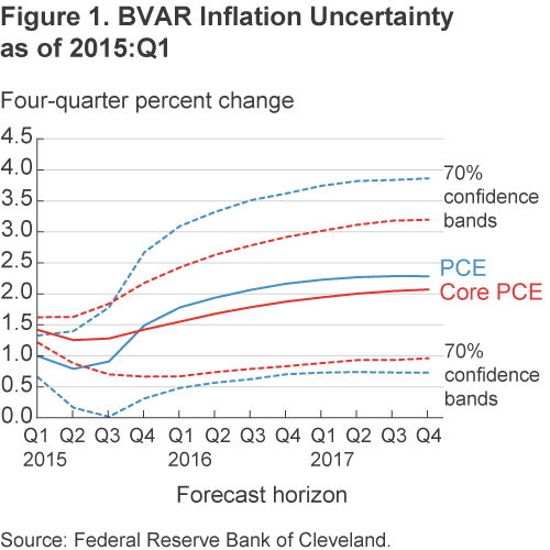
Wider confidence bands equate to greater uncertainty about the potential range of outcomes. Notably, the bands for PCE inflation are always wider than the bands for core PCE inflation, because PCE inflation is subject to more volatile shocks (think energy prices) than core PCE inflation. This naturally makes PCE inflation harder to predict than core PCE inflation.
To come up with a single quantitative measure of forecast uncertainty at a given point in time, we look at the width of the 70 percent confidence interval eight quarters into the future. The trailing four-quarter inflation rate that is eight quarters in the future is also known as 1-year/1-year-forward inflation. This is a fairly representative point in the future, and it allows for near-term events to have partially played out. Given that monetary policy is usually thought to operate with long and variable lags, in the words of Milton Friedman, it may also be a horizon that is of interest to monetary policymakers. For our forecast made in 2015:Q1 using the BVAR model, for example, we would estimate that inflation forecast uncertainty would be 2.1 percentage points for core PCE inflation and 2.9 percentage points for PCE inflation.
The Evolution of Inflation Forecast Uncertainty
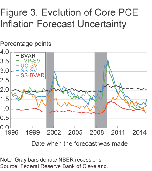
Using this framework, we can place current inflation forecast uncertainty into context, both across models and across time. To do this comparison accurately, we recursively generate out-of-sample forecast uncertainty using real-time data. That is, for each point in time, we look at the dataset that would have actually been available to a forecaster using a particular model; we construct the forecasts coming from that model for inflation one-year/one-year-forward to measure forecast uncertainty; and then we move on to the next period and repeat the exercise.13 Our earliest forecasts come from data that were available in 1996:Q1; our last forecasts use data available as of 2015:Q1. In all cases, our forecasts come directly from the models and do not take advantage of any near-term conditioning from outside sources.14 Figure 2 shows the evolution of PCE inflation forecast uncertainty, and Figure 3 shows the evolution of core PCE inflation forecast uncertainty.15
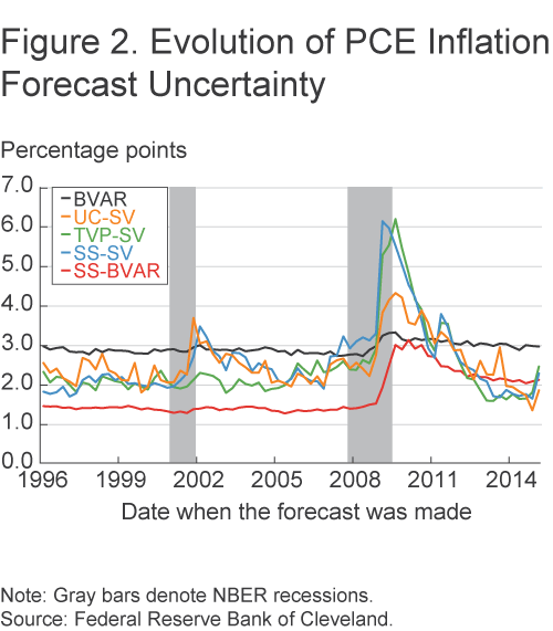
Inflation forecast uncertainty is generally highest in the BVAR model. This result is intuitive, because the construction of the forecasts is partly influenced by the volatile inflation experience of the 1970s, which is part of the estimation sample. The Great Recession has only a moderate impact on forecast uncertainty in this model because it is only one part of a very long time series. While the effects of the Great Recession on uncertainty in this model are not very large, they do cast a long shadow: uncertainty is still slightly elevated due to the experiences of the Great Recession but it is trending lower.
By contrast, inflation forecast uncertainty is generally lowest in the SS-BVAR model. The sample period for this model begins in the mid-1980s, coinciding with the Great Moderation; inflation was difficult to predict during this time, but it was not nearly as volatile as it was in the 1970s. Because the Great Recession was a large event in this short historical time series, it has a larger impact on inflation forecast uncertainty than in the BVAR model. For PCE inflation, forecast uncertainty has diminished since the Great Recession, but it has not yet reached its pre-Great Recession levels. For core inflation, the effects of the Great Recession have been largely undone.
Forecast uncertainty moves around a considerable amount based on the models with stochastic volatility. Intuitively, stochastic volatility allows this class of models to rapidly capture the changing nature of the shocks hitting the economy; time-varying parameters can further capture structural changes as well. The three models with stochastic volatility exhibit relatively similar movements in forecast uncertainty. One spike in uncertainty occurred around the 2001 recession and the September 11, 2001, terrorist attacks. A second spike in uncertainty occurred around the Great Recession. In all cases, because volatilities can and do rapidly change in these types of models in response to the incoming data, the forecast uncertainty associated with the Great Recession is a distant memory.
Finally, we can rank current inflation forecast uncertainty as of 2015:Q1 relative to other readings since 1996, and we can quantitatively compare current uncertainty to its peak level around the Great Recession, shown in Table 2. In four of our five models, PCE inflation forecast uncertainty is currently in the normal to somewhat elevated range by historical norms of the last 20 years, residing in the 51st through 77th percentiles.16 By contrast, core inflation forecast uncertainty is relatively low: it is essentially near historical norms according to two models (in the 58th through 64th percentiles) and quite low according to the other three (in the 4th through 34th percentiles). Across almost all of our models, inflation forecast uncertainty today is dramatically below its levels from around the Great Recession, having fallen by as much as two-thirds in some cases.17
Table 2. Current Inflation Uncertainty in Perspective
| Current percentile | ||
|---|---|---|
| PCE inflation | Core PCE inflation | |
| BVAR | 68 | 64 |
| SS-BVAR | 77 | 58 |
| UC-SV | 6 | 4 |
| SS-SV | 51 | 34 |
| TVP-SV | 75 | 14 |
| Change in uncertainty since the Great Recession peak (percent) | ||
| PCE inflation | Core PCE inflation | |
| BVAR | 11 | 12 |
| SS-BVAR | 32 | 33 |
| UC-SV | 60 | 65 |
| SS-SV | 63 | 56 |
| TVP-SV | 57 | 50 |
Notes: Current forecast uncertainty is based on data through 2014:Q4. The percentiles show how current forecast uncertainty ranks compared with the forecast uncertainty starting in 1996:Q1.
Conclusion
Using a range of statistical models, we examine the outlook for inflation. These models generally predict that inflation will rise from its recent subdued readings. Our models also allow us to measure the uncertainty surrounding the inflation outlook. Doing so reveals that inflation forecast uncertainty today is perhaps somewhat elevated compared with the norms of the last 20 years, while forecast uncertainty for core inflation is relatively low compared with the same period. But if we focus on the recent past, inflation forecast uncertainty as of the first quarter of 2015 is much lower than it was around the Great Recession.
Footnotes
- See http://www.federalreserve.gov/newsevents/press/monetary/20150318a.htm. Return to 1
- For a policymaker’s perspective, see Mester (2015). Return to 2
- Atkeson and Ohanian (2001), among others, advocate for forecasting future inflation with the recent past, and this model serves as a useful benchmark for forecast accuracy comparisons. Stock and Watson (2002) is one example of a factor model applied to inflation forecasting. Faust and Wright (2013) provide a broad overview of inflation forecast approaches and their relative merits. Return to 3
- Real GDP and real PCE enter the model in log levels. Unit labor cost growth is defined as growth in the employment cost index for private workers less growth in nonfarm business sector labor productivity. Our two inflation measures, PCE inflation and core PCE inflation, are modeled as deviations from a slow-moving inflation trend. The trend for core PCE inflation is the long-term inflation expectations series from the Federal Reserve Board of Governor’s FRB/US econometric model, denoted PTR. For PCE inflation, we use core PCE inflation for the trend. In autoregressive models, specifying inflation as a deviation from trend has been found to improve forecast accuracy (see, e.g., Kozicki and Tinsley 2001, Clark 2011, and Zaman 2013). Return to 4
- Alesi, Ghysels, Onorante, and Potter (2014) and Andreou, Ghysels, and Kourtellos (2012) present some evidence that the inclusion of financial variables helps improve forecasting accuracy around the Great Recession. In our SS-BVAR, we split unit labor costs into ECI growth and productivity growth. Real GDP, real PCE, and the S&P 500 also enter the model in growth rates. Return to 5
- Strachan and van Dijk (2013) present evidence of a structural break in VAR modeling around 1984. Return to 6
- While Stock and Watson (2007) calibrate γ=0.2 in the shock process that drives the stochastic volatilities, we estimate this parameter. Return to 7
- Faust and Wright (2013) show that including accurate nowcast information dramatically improves inflation forecasting performance, especially in the near term; see also the results in Krueger et al. (2014). To this end, the inflation nowcasting model developed by Knotek and Zaman (2014) could be used to generate nowcasts, and these nowcasts can be used to condition near-term inflation outcomes with an eye toward improving longer-term inflation forecast accuracy. In all the exercises we present, however, we focus solely on unconditional forecasting exercises that omit nowcasts. Return to 8
- Model averaging can deliver highly accurate inflation forecasts; see Wright (2009). For density forecasts generated by model averaging, see Mitchell and Wallis (2011). Return to 9
- In addition, uncertainty arises because we do not know the model’s “true” parameters and must estimate them. That estimation creates sampling error in the parameters, which adds to uncertainty around the forecast. Return to 10
- Knotek and Zaman (2013) use this feature of the BVAR model to compute the probabilities of certain events that might have triggered a monetary policy response under threshold and floor scenarios. Return to 11
- Plugging in values from the inflation nowcasts on the Cleveland Fed’s website suggests that four-quarter PCE inflation in 2015:Q1 is likely to fall below the lower 70 percent confidence band, further illustrating the perils of inflation forecasting. Return to 12
- Our real-time dataset uses observations from the databases maintained by the Federal Reserve Banks of Philadelphia and St. Louis. Pseudo real-time data were used sparingly to fill in missing observations. The timing of real-time observations within a quarter generally matches survey dates from the Philadelphia Fed’s Survey of Professional Forecasters. Return to 13
- As noted above, not imposing nowcasts may reduce the accuracy of our forecasts and increase forecast uncertainty, but the use of a 1-year/1-year-forward horizon helps to mitigate this result. Additionally, this exercise raises some questions about how to treat the period of the zero lower bound on nominal interest rates: for models that include the federal funds rate, the forecasts would have predicted negative values at certain points in time, and there is nothing to prevent interest rates from falling below zero in the models. As a check, we re-ran our models from 2008:Q4 through the present and conditioned the path of the federal funds rate to match the path predicted by the survey respondents in the Blue Chip Economic Indicators survey, because these forecasts respected the zero lower bound. This conditional exercise generated results similar to those in the figure. To maximize historical comparability, our figures show the unconditional forecasts coming from the models. Return to 14
- The gray bars in the figure denote recessions as defined by the National Bureau of Economic Research (NBER). Return to 15
- The uncertainty percentiles reflect an ordered ranking of inflation uncertainty outcomes; e.g., the 2015:Q1 BVAR uncertainly level is the 52nd largest out of 77 readings, putting it into the 68th percentile. The interpretation is similar if instead we assume that inflation forecast uncertainty since 1996 has followed a log-normal distribution. Return to 16
- The Summary of Economic Projections (SEP) made by members of the Federal Open Market Committee contains information on the typical amount of uncertainty surrounding consumer price inflation projections. This information is based on average historical forecast errors from the prior 20 years coming from forecasts made by various private and government forecasters; e.g., see http://www.federalreserve.gov/monetarypolicy/files/fomcminutes20141217.pdf and the associated working paper by Reifschneider and Tulip (2007). This approach provides a somewhat different interpretation of “normal” forecast uncertainty compared with our approach. In principle, the SEP methodology could be used to construct the evolution of forecast uncertainty as we have done, by using a rolling 20-year window and finding the average historical forecast errors at each step as the window moves through time from 1996 to the present. Return to 17
References
- Alessi, Lucia, Eric Ghysels, Luca Onorante, Richard Peach, and Simon Potter (2014) “Central Bank Macroeconomic Forecasting during the Global Financial Crisis: The European Central Bank and Federal Reserve Bank of New York Experiences,” Federal Reserve Bank of New York Staff Report No. 680.
- Andreou, Elena, Eric Ghysels, and Androus Kourtellos (forthcoming) “Should Macroeconomic Forecasters Use Daily Financial Data and How?” Journal of Business and Economic Statistics.
- Atkeson, Andrew and Lee E. Ohanian (2001) “Are Phillips Curves Useful for Forecasting Inflation?” Federal Reserve Bank of Minneapolis, Quarterly Review (Winter): 2–11.
- Clark, Todd E. (2011) “Real-Time Density Forecasts from Bayesian Vector Autoregressions with Stochastic Volatility,” Journal of Business and Economic Statistics 29(3): 327-41.
- Cogley, Timothy, and Thomas J. Sargent (2005) “Drifts and Volatilities: Monetary Policies and Outcomes in the Post WWII U.S.” Review of Economic Dynamics 8(2): 262-302
- D’Agostino, Antonello, Luca Gambetti, and Domenico Giannone (2013) “Macroeconomic Forecasting and Structural Change,” Journal of Applied Econometrics 28(1): 82-101.
- Faust, Jon and Jonathan H. Wright (2013) “Forecasting Inflation” in Graham Elliott and Allan Timmermann, eds., Handbook of Economic Forecasting, vol. 2, Elsevier: North Holland.
- Knotek, Edward S., II and Saeed Zaman (2014) “Nowcasting U.S. Headline and Core Inflation,” Federal Reserve Bank of Cleveland, working paper 2014-03.
- Knotek, Edward S., II and Saeed Zaman (2013) “When Might the Federal Funds Rate Lift Off? Computing the Probabilities of Crossing Unemployment and Inflation Thresholds (and Floors)” Federal Reserve Bank of Cleveland, Economic Commentary 2013-19.
- Kozicki, Sharon and P.A. Tinsley (2001) “Shifting Endpoints in the Term Structure of Interest Rates” Journal of Monetary Economics 47(3): 613-52.
- Krueger, Fabian, Todd E. Clark, and Francesco Ravazzolo (2014) “Using Entropic Tilting to Combine BVAR Forecasts with External Nowcasts,” Federal Reserve Bank of Cleveland, working paper no. 14-39.
- Mester, Loretta J. (2015) “The Outlook for the Economy and Monetary Policy Communications” speech delivered at the 31st Annual NABE Economic Policy Conference.
- Mitchell, James and Kenneth F. Wallis (2011) “Evaluating Density Forecasts: Forecast Combinations, Model Mixtures, Calibration and Sharpness” Journal of Applied Econometrics 26(6): 1023-1040.
- Reifschneider, David and Peter Tulip (2007) “Gauging the Uncertainty of the Economic Outlook from Historical Forecasting Errors” Finance and Economics Discussion Series working paper number 2007-60.
- Stock, James H. and Mark W. Watson (2002) “Macroeconomic Forecasting Using Diffusion Indexes” Journal of Business and Economic Statistics 20(2): 147-162.
- Stock, James H. and Mark W. Watson (2007) “Why Has U.S. Inflation Become Harder to Forecast?” Journal of Money, Credit and Banking 39(S1): 3-33.
- Strachan, Rodney W. and Herman K. van Dijk (2013) “Evidence on Features of a DSGE Business Cycle Model from Bayesian Model Averaging” International Economic Review 54(1): 385-402.
- Villani, Mattias (2009) “Steady-State Priors for Vector Autoregressions” Journal of Applied Econometrics 24(4): 630-50.
- Wright, Jonathan (2009) “Forecasting U.S. Inflation by Bayesian Model Averaging” Journal of Forecasting 28(2): 131-44.
- Zaman, Saeed (2013) “Improving Inflation Forecasts in the Medium to Long Term” Federal Reserve Bank of Cleveland, Economic Commentary 2013-16.
Suggested Citation
Clark, Todd E., Edward S. Knotek II, and Saeed Zaman. 2015. “Measuring Inflation Forecast Uncertainty.” Federal Reserve Bank of Cleveland, Economic Commentary 2015-03. https://doi.org/10.26509/frbc-ec-201503
This work by Federal Reserve Bank of Cleveland is licensed under Creative Commons Attribution-NonCommercial 4.0 International

