

- Share
School Quality and Housing Affordability: Who Occupies Housing in the Best-Performing School Districts?
High-performing school districts attract families seeking quality education, but housing in these areas is often expensive and limited. One potential contributor is older households—many of whom may no longer have children in local schools—aging in place. In this Economic Commentary, we examine how different household types are distributed across school districts of varying education quality and affordability. We find that while older households do occupy a modestly larger share of housing in high-performing, expensive districts relative to high-performing, more-affordable districts, their presence does not result in relatively lower housing turnover. Instead, affordability challenges reflect broader patterns: higher-income households of all types compete for housing in the best-performing school districts. These findings suggest that policies aimed solely at encouraging older households to downsize are unlikely to substantially improve access to quality school districts.


The views authors express in Economic Commentary are theirs and not necessarily those of the Federal Reserve Bank of Cleveland or the Board of Governors of the Federal Reserve System. The series editor is Tasia Hane. This paper and its data are subject to revision; please visit clevelandfed.org for updates.
Introduction
Because public schools in the United States are funded in part by local property taxes and because school access is determined by residential location, neighborhoods with higher housing costs tend to have higher-performing schools. School quality is therefore an amenity for which households with children are willing to pay a premium (Black, 1999; Hörnig and Schäfer, 2025), and both house prices and rents are systematically higher in areas with high-performing school districts (see Figures 1a and 1b). This creates a barrier to entry: the neighborhoods with the most beneficial educational infrastructure have the most expensive housing costs for families. Competition for housing in these districts is broad; it extends beyond parents with school-aged children to include young professionals who target these areas for their investment security and older households and empty-nesters who choose to age in place rather than downsize.
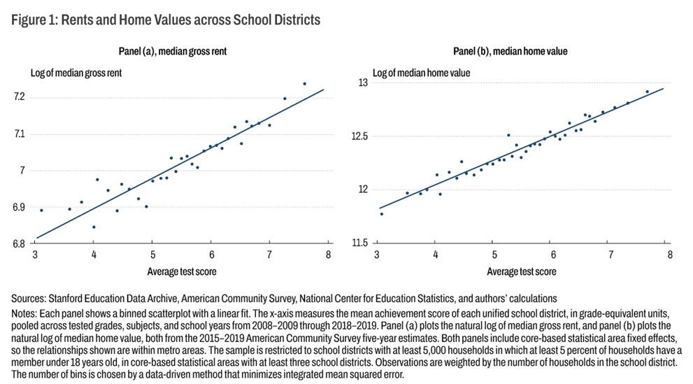
As housing affordability has become an increasingly pressing policy concern, attention has also turned to factors that may limit housing availability and in turn further drive up housing prices and rents. One such factor is older households’ aging in place. These households often remain in larger homes years after their children have left. If they were to downsize, the homes could become available to larger, younger families. One estimate indicates that had older households continued to relocate at their 2019 levels, an additional 500,000 bedrooms would have been freed up, not as new housing supply, but as a reallocation of existing stock toward households with greater space needs (Shampine, 2025).1 If this dynamic is widespread, families with school-aged children, or young adults hoping to start families, may be systematically priced out of the areas with the best educational opportunities. Understanding whether this pattern exists in the data and measuring its scale is therefore vital for both housing and education policy.
In this Economic Commentary, we look to see whether these geographic concentrations of different household types are visible in the data. We categorize school districts within metro areas by both quality—measured using average test scores—and affordability—measured using the ratio of median home values to local household median income. We then see where different household types choose to live. Specifically, we examine whether families with school-aged children occupy a smaller share of housing in the highest-performing, most-expensive school districts and whether older empty-nester households account for a disproportionately larger share of households within these districts.2
We find that older households do occupy a modestly larger share of housing in high-quality, expensive districts, rising from about a quarter of households in low-quality districts to almost 29 percent in the least-affordable high-quality districts. However, affordability challenges in high-quality school districts appear driven by broader income sorting patterns rather than by older households alone. Higher-income households of all types concentrate in better school districts, with this pattern most pronounced for families with children. Families with children in less-affordable (measured using house prices relative to income), high-quality districts have incomes more than double those of families in low-quality but still unaffordable districts. Additionally, young single-person households make up a larger share of residents in less-affordable areas regardless of school quality, suggesting that competition for housing in expensive districts extends beyond families seeking good schools.
Data
We use data from the American Community Survey (ACS) five-year estimates for 2015–2019, aggregated to the unified school district level. Unified school districts provide both elementary and secondary education and typically correspond to the area served by a single public school system. From the ACS, we use measures of household composition, tenure, median household income, median home values, median rents, homeownership rates, and mobility. Specifically, we examine the share of households with children under 18 years old, the share of households headed by someone 65 or older, the share of one-person households, median income by household type, homeownership rates by household type, and the share of people who moved in the last year, by tenure and by age.3
To measure educational quality across school districts, we use data from the Stanford Education Data Archive (SEDA). SEDA provides standardized measures of academic achievement and learning rates for school districts across the United States, derived from state standardized test scores in math and reading/language arts. The data are placed on a common scale that allows for comparisons across districts and states and over time. We use the pooled geographic-district mean achievement score in grade-equivalent units from SEDA 6.0, a measure of average achievement across tested grades, subjects, and years from the 2008–2009 school year through the 2018–2019 school year (11 years). We match SEDA to the ACS unified school district tabulations using the seven-digit National Center for Education Statistics (NCES) district identifier. We use geographic concordances (data translation tools that match different regional boundaries) from NCES education demographic and geographic estimates to associate each school district with one core-based statistical area (CBSA).4
We limit our analysis to unified school districts for which the ACS publishes information on both median income and median house values in CBSAs comprising at least three school districts. We further restrict our dataset to school districts with at least 5,000 households in which at least 5 percent of households have a member under 18 years old. This restriction removes age-restricted senior living communities from our analysis. We conduct our analysis on a within-CBSA basis, as households generally search for school districts within a given metro area. We examine three main household groups: households with members under 18 years old; households headed by someone aged 65 or older, many of whom are empty-nesters whose children have moved out; and single-person households headed by someone younger than 65.
We divide school districts into nine bins based on school quality and housing affordability measured using the ratio of median house value to median income from the ACS. Within each CBSA, we separate school districts into household-weighted terciles of school quality using the mean achievement score from SEDA. The bottom third are classified as low quality, the middle third as medium quality, and the top third as high quality. We then divide school districts into household-weighted terciles of affordability using the median home value to median income ratio from the ACS. These terciles are similarly labeled as low, medium, and high cost. Each combination of school quality and affordability tercile defines one bin, yielding nine bins in total. We remove CBSAs for which this procedure does not result in nine distinct bins. Our final sample includes 178 CBSAs, which collectively are home to 58.6 million households.
Results
While our binning procedure divides school districts into terciles within each CBSA, the resulting bins vary considerably in the number of households they contain. Table 1 shows the number of households (in millions) in each quality-affordability bin. The low-quality, low-cost bin contains the most households—11.5 million—while the low-quality, high-cost bin contains the fewest, at 4.1 million. High-quality districts are more evenly distributed across affordability terciles, with between 4.7 million and 5.9 million households in each bin.
Table 1: Number of Households by School Quality and Affordability (Millions)
| House value/income | ||||
| School quality | Low | Medium | High | All |
| Low | 11.5 | 9.1 | 4.1 | 24.7 |
| Medium | 7.6 | 5.6 | 4.5 | 17.7 |
| High | 5.6 | 4.7 | 5.9 | 16.2 |
| All | 24.7 | 19.4 | 14.5 | 58.6 |
The main results of our analysis are displayed in Table 2. On the left-hand side of this table, we show the composition of each bin: the percentage of households in each bin that have children, are aged 65 or older, or are single-person households younger than 65. On the right-hand side, we show the distribution of each household type across bins. These numbers reflect the percent of all households with children, households aged 65 or older, and single-person households younger than 65 in our sample that reside in each bin. The columns (rows) labeled “All” contain the numbers for the respective affordability (quality) bins across all three of the quality (affordability) bins. The bottom-right cells of the composition table contain the overall aggregate shares of each household type in the sample.
Table 2: Household Composition and Distribution by School Quality and Affordability
| School quality | Composition (%) | Distribution (%) | |||||||
| House value/income | |||||||||
| Low | Med | High | All | Low | Med | High | All | ||
| Low |
HH w/kids | 31.8 | 30.3 | 27.5 | 30.5 | 19.6 | 14.5 | 5.9 | 40.0 |
| 65+ HH | 25.3 | 24.8 | 25.4 | 25.2 | 19.6 | 14.2 | 6.3 | 40.1 | |
| 1-person | 28.8 | 30.0 | 33.5 | 30.0 | 21.2 | 19.2 | 10.2 | 50.6 | |
| Medium |
HH w/kids |
32.3 | 29.8 | 27.5 | 30.3 | 14.0 | 9.4 | 6.5 | 29.9 |
| 65+ HH | 26.1 | 27.3 | 27.4 | 26.8 | 13.4 | 9.9 | 7.7 | 31.0 | |
| 1-person | 24.9 | 27.4 | 29.7 | 26.9 | 10.5 | 8.7 | 9.0 | 28.2 | |
| High |
HH w/kids |
35.4 | 33.4 | 30.7 | 33.1 | 11.1 | 8.9 | 10.1 | 30.1 |
| 65+ HH |
25.3 | 27.1 | 28.7 | 27.0 | 9.3 | 8.3 | 11.3 | 28.9 | |
| 1-person |
21.8 | 23.7 | 26.3 | 24.0 | 6.7 | 5.9 | 8.7 | 21.3 | |
| All |
HH w/kids | 32.8 | 30.9 | 28.8 | 31.2 | 44.7 | 32.8 | 22.4 | 100.0 |
| 65+ HH | 25.6 | 26.1 | 27.3 | 26.2 | 42.3 | 32.4 | 25.2 | 100.0 | |
| 1-person | 26.0 | 27.7 | 29.4 | 27.4 | 38.3 | 33.8 | 27.8 | 100.0 | |
Notes: Composition shows the share of households within each cell that are of a given type. Distribution shows the share of all households of a given type that live in each cell. Cell values are weighted across districts. “All” rows and columns show weighted averages across cells for composition and sums across cells for distribution.
Two patterns emerge from the composition data on the left-hand side of Table 2. Within each affordability category, the share of households with children is almost always increasing with school quality. In the most affordable districts, 31.8 percent of households in low-quality districts have children, while in high-quality districts 35.4 percent have children. However, within each school quality category, the share of households with children is decreasing as housing becomes more unaffordable. For the highest-quality school districts, 35.4 percent of households have children in the most-affordable districts, compared to 30.7 percent in the least-affordable districts. By comparison, 31.2 percent of all households in our data are households with children. The distribution data on the right-hand side of Table 2 reveal that the largest concentration of households with children, 19.6 percent, lives in low-quality, low-cost school districts, compared with 10.1 percent who live in high-quality, high-cost districts. Overall, 40.0 percent of households with children live in low-quality districts, while 30.1 percent live in high-quality districts.
The patterns for older households in Table 2 differ notably from those of households with children. The share of households aged 65 and older is relatively flat across affordability bins for low-quality school districts and rises only modestly in medium-quality districts (26.1 to 27.4 percent). However, for high-quality districts, it increases from 25.3 percent in the most affordable areas to 28.7 percent in the least affordable areas. Households over age 65 comprise 26.2 percent of households overall. This provides some evidence that older empty-nesters occupy a disproportionate share of housing in high-quality, high-cost school districts. Similar to households with children, older households are also most concentrated in low-quality, low-cost districts, a situation reflecting the overall distribution of housing across bins.
The pattern for single-person households in Table 2 also differs. Unlike older households, whose concentration in high-cost areas is most pronounced in high-quality districts, the share of one-person households increases with house value-to-income ratios across all school quality categories. While perhaps surprising, these same unaffordable areas are likely those with the most opportunities for young professionals seeking access to urban amenities and labor markets (Diamond, 2016).
Table 3 shows the median income of each household type across bins. Incomes for all household types are generally increasing both across affordability bins and across school-quality bins. The main exception is in the lowest-quality school districts, in which incomes of households with children and older households are both higher in the lower-cost districts, perhaps because these districts offer similar school quality regardless of housing costs, giving higher-income households less incentive to pay a premium. The increase in income with school quality is most dramatic for households with children; in the lowest-quality school districts, the median income for households with children is below $60,000, while in the highest-quality districts that number roughly doubles. The increases in income with school quality for older and one-person households are less severe.
Table 3: Median Household Income by Type, School Quality, and Affordability ($1,000s)
| School quality | House value/income | ||||
| Low | Med | High | All | ||
| Low |
Households with children | 59.2 | 57.3 | 55.4 | 58.0 |
| 65+ households | 43.5 | 43.3 | 40.5 | 42.9 | |
| 1-person HH | 30.7 | 34.0 | 34.0 | 32.6 | |
| All households | 55.9 | 56.9 | 54.9 | 56.1 | |
| Medium |
Households with children |
82.8 | 84.1 | 92.0 | 85.2 |
| 65+ households | 49.4 | 52.3 | 52.5 | 51.1 | |
| 1-person HH | 36.6 | 38.7 | 43.1 | 39.3 | |
| All households |
72.4 | 72.1 | 75.0 | 73.0 | |
| High |
Households with children |
110.5 | 123.8 | 123.8 | 118.9 |
| 65+ households |
58.3 | 59.6 | 63.3 | 60.6 | |
| 1-person HH |
42.8 | 44.4 | 45.4 | 44.3 | |
| All households |
91.1 | 95.6 | 91.7 | 92.6 | |
| All |
Households with children | 79.3 | 83.0 | 96.7 | 84.4 |
| 65+ households | 48.6 | 50.3 | 54.3 | 50.6 | |
| 1-person HH | 34.4 | 37.0 | 40.5 | 37.0 | |
| All households |
68.9 | 70.6 | 76.1 | 71.3 | |
Notes: Cell values show weighted average of district-level median incomes, weighted by household counts. “All” rows and columns show weighted averages across cells. 1-person HH income includes all ages (data not available separately for under 65).
High-quality school districts also have higher homeownership rates, as shown in Table 4. This is the case for all household types, but it is, again, most dramatic for households with children; these households have around a 40 percent to 46 percent homeownership rate in low-quality districts and close to a 70 percent homeownership rate in high-quality districts. While older households generally have higher homeownership rates across all bins, their homeownership rates do not vary as substantially with school-district quality.
Table 4: Homeownership Rates by Type, School Quality, and Affordability (%)
| School quality | House value/income | ||||
| Low | Med | High | All | ||
| Low |
Households with children | 46.4 | 40.6 | 39.6 | 43.3 |
| 65+ households | 76.1 | 69.7 | 66.3 | 72.3 | |
| 1-person HH (<65) | 41.6 | 32.1 | 30.4 | 35.7 | |
| All households | 59.5 | 49.6 | 46.7 | 53.7 | |
| Medium |
Households with children |
60.5 | 57.9 | 56.2 | 58.7 |
| 65+ households | 81.5 | 78.8 | 74.2 | 78.8 | |
| 1-person HH (<65) | 52.8 | 45.5 | 35.8 | 45.1 | |
| All households |
71.2 | 66.3 | 57.8 | 66.3 | |
| High |
Households with children |
68.3 | 71.1 | 68.0 | 69.0 |
| 65+ households |
82.7 | 80.9 | 79.1 | 80.8 | |
| 1-person HH (<65) |
54.5 | 51.4 | 43.5 | 49.2 | |
| All households |
74.3 | 73.9 | 68.9 | 72.2 | |
| All |
Households with children | 56.2 | 53.8 | 57.1 | 55.7 |
| 65+ households | 79.3 | 75.4 | 74.4 | 76.8 | |
| 1-person HH (<65) | 46.9 | 38.9 | 36.2 | 41.2 | |
| All households |
66.5 | 60.3 | 59.2 | 62.6 | |
Notes: Cell values show weighted homeownership rates across districts, calculated as total owners divided by total households. “All” rows and columns show weighted averages across cells.
To assess whether older empty-nesters are limiting turnover of the existing housing stock, Table 5 reports the share of people who moved in the last year within each quality-affordability bin, separately for people living in owner-occupied housing, all people living in households, and all people aged 65 and older. The moving rate of people in owner-occupied housing units is close to 8 percent for all bins. However, overall mobility is lower in high-quality districts: it is 12.8 percent on average versus 15.1 percent in low-quality districts. This is driven by the differences in homeownership rates across these areas and by the fact that renters move more frequently than homeowners. Among people aged 65 and older, the mobility rate is between 6.4 and 7.4 percent in every bin, and it is not lower in high-quality districts (6.9 percent) than in low-quality districts (6.8 percent).5 Within high-quality districts, 65+ mobility is essentially flat as costs rise (6.8 to 6.9 percent), even though the share of households aged 65 and older rises from 25.3 to 28.7 percent. Most older households own their homes (77 percent overall and 81 percent in high-quality districts; Table 4), so the stable mobility rate of people in owner-occupied housing across bins points in the same direction. Taken together, these results do not suggest that older households are limiting turnover of the housing stock in high-quality, high-cost districts.
Table 5: Average Turnover by School Quality and Affordability (%)
| School quality | House value/income | ||||
| Low | Med | High | All | ||
| Low |
Homeowners | 8.0 | 7.5 | 8.3 | 7.8 |
| Overall | 14.8 | 14.7 | 17.2 | 15.1 | |
| Age 65+ | 6.8 | 6.6 | 7.4 | 6.8 | |
| Medium |
Homeowners |
7.9 | 7.7 | 8.0 | 7.9 |
| Overall | 12.4 | 13.2 | 15.4 | 13.4 | |
| Age 65+ | 6.4 | 6.5 | 6.8 | 6.5 | |
| High |
Homeowners |
8.1 | 7.9 | 7.9 | 8.0 |
| Overall |
12.4 | 12.3 | 13.8 | 12.8 | |
| Age 65+ |
6.8 | 6.9 | 6.9 | 6.9 | |
| All |
Homeowners | 8.0 | 7.7 | 8.0 | 7.9 |
| Overall | 13.5 | 15.7 | 15.2 | 13.9 | |
| Age 65+ | 6.7 | 6.6 | 7.0 | 6.7 | |
Note: Turnover rate is the percentage of people age 1 and over who moved in the past year. Cell values show weighted averages across districts, weighted by population.
“All” rows and columns show weighted averages across cells. Homeowners and Overall cover people in owner-occupied and all households (B07013). Age 65+ covers people 65 and over (B07001), including group quarters.
Conclusion
Households with children appear to be drawn to high-performing school districts, but cluster in those where housing costs are most affordable. The districts that are both high-quality and high-cost attract higher-income households across all types, including young professionals without children. While older households occupy a modestly larger share of housing in these expensive, high-quality areas, they do not appear to limit turnover. These patterns suggest that the challenge of accessing high-quality school districts is driven by a combination of income sorting and competition from multiple household types rather than solely by empty-nesters’ aging in place.
References
- Black, Sandra E. 1999. “Do Better Schools Matter? Parental Valuation of Elementary Education.” Quarterly Journal of Economics 114(2): 577–599. jstor.org/stable/2587017.
- Diamond, Rebecca. 2016. “The Determinants and Welfare Implications of US Workers’ Diverging Location Choices by Skill: 1980–2000.” American Economic Review 106(3): 479–524. doi.org/10.1257/aer.20131706.
- Hörnig, Lukas, and Max Schäfer. 2025. “The Value of School Choice Opportunities.” Labour Economics 95: 102742. doi.org/10.1016/j.labeco.2025.102742.
- Jones, John, Yue Li, and Urvi Neelakantan. 2024. “The Living Arrangements of Older Households.” Federal Reserve Bank of Richmond, Economic Brief, 24-33. richmondfed.org/publications/research/economic_brief/2024/eb_24-33.
- Kim, Jinyhup. 2024. “Aging, Housing Prices, and Young Adults’ Homeownership.” Cities 149: 104914. doi.org/10.1016/j.cities.2024.104914.
- Shampine, Samantha. 2025. “Housing Trends: Older Households Are Moving Less, and Multigenerational Living Is Rising.” Federal Reserve Bank of Boston, Current Policy Perspectives, 25-9. bostonfed.org/publications/current-policy-perspectives/2025/housing-trends-older-households-moving-less-multigenerational-living-rising.aspx.
Endnotes
- Other recent work by Kim (2024) and Jones et al. (2024) also shows evidence that older households’ desire to age in place may increase affordability pressures for younger households. Return to 1
- For the purposes of this Economic Commentary, we focus on describing patterns that existed prior to the COVID-19 pandemic, as changes to in-person schooling during the pandemic make it more complicated to assess school performance using test scores in the cross-section. We also do not control for other aspects of high-performing school districts that increase their appeal as a place to live such as libraries, parks, or community centers. This is by design. The purpose of this Economic Commentary is to see how stark the distribution of household types is across different school districts, not to ascertain the reasons why they differ. Return to 2
- These come from ACS tables B11005 (households by presence of people under 18), B25064 (median gross rent), B25077 (median house value), B19013 (median household income), B25115 (tenure by family type), B25116 (tenure by household size and age), B11016 (household type), B19125 (median income for families with and without kids), B19049 (median income by household age), B19019 (median income by household size), B07013 (tenure by migration in last year), B07001 (geographical mobility by age), and B09020 (household relationship for the population 65 and over). Return to 3
- School districts that cross CBSA borders are assigned the CBSA that accounts for the majority of their land area. Return to 4
- About 3 percent of people aged 65 and older in our sample live in group quarters, such as nursing homes. Because the share of older people living in group quarters varies little across bins (2.3 to 3.8 percent; ACS table B09020), any effect on the 65+ mobility rates is likely similar across cells. Return to 5
Suggested Citation
Loewenstein, Lara, and Paul S. Willen. 2026. “School Quality and Housing Affordability: Who Occupies Housing in the Best-Performing School Districts?” Federal Reserve Bank of Cleveland, Economic Commentary 2026-27. https://doi.org/10.26509/frbc-ec-202627
This work by Federal Reserve Bank of Cleveland is licensed under Creative Commons Attribution-NonCommercial 4.0 International


