- Share
Have Inflation Dynamics Changed?
Using a flexible statistical model to project inflation outcomes into the future, this Commentary finds that the most likely path for inflation based on recent inflation dynamics is generally similar to what would have been expected given inflation dynamics in the late 1990s, but there is more uncertainty around the forecast now than in the late 1990s.
The views authors express in Economic Commentary are theirs and not necessarily those of the Federal Reserve Bank of Cleveland or the Board of Governors of the Federal Reserve System. The series editor is Tasia Hane. This paper and its data are subject to revision; please visit clevelandfed.org for updates.
After rising in the second half of 2016 and in the early part of 2017, inflation as measured by the price index for personal consumption expenditures (PCE) began to reverse course unexpectedly. While PCE inflation has been below 2 percent for most of the expansion following the Great Recession, its recent decline came in the midst of a low and falling unemployment rate, stable oil prices, and a depreciating dollar. These forces would not ordinarily be expected to put downward pressure on inflation. This situation has posed something of a “mystery” for monetary policymakers (see, e.g., Yellen 2017b). Seeking to explain this disconnect between inflation and its fundamental drivers, some economists have raised questions about whether inflation dynamics have recently changed, perhaps as a result of ongoing globalization, technological innovation, or shifts in the competitive environment related to the internet, among other factors.1
In this Commentary, we look at inflation through the lens of a flexible statistical model that can capture time-variation in inflation dynamics and in the relationship between inflation and unemployment. Using this model, we generate two sets of inflation forecasts. The first forecast is based on the most recent behavior of inflation and the unemployment rate. In the second forecast, we assume that inflation dynamics are governed by the behaviors we saw in the late 1990s—another period in which both the unemployment rate and inflation were notably low, but also one in which globalization and internet commerce may have been putting less downward pressure on inflation. In terms of the most likely paths going forward, the point forecasts for inflation and unemployment from these two approaches are generally similar—and, if anything, the projection based on recent inflation dynamics calls for a more rapid rise of inflation to 2 percent today than would have been the case in the late 1990s. But there is more uncertainty surrounding the point forecasts now than in the late 1990s, consistent with an economy that is now subject to larger shocks and a looser relationship between inflation and unemployment than in the past.
Capturing Time Variation
To adequately address whether inflation dynamics may have changed and what those changes imply for the inflation outlook, we need a model for forecasting inflation, a method for estimating the model that can pick up changes in inflation dynamics, and a suitable base period for comparison.
For the model, we have chosen a bivariate vector autoregression (VAR) using quarterly data on the unemployment rate and core PCE inflation, which excludes food and energy prices. The Phillips curve typically relates inflation to the unemployment rate. While our model is related to the literature on Phillips curves, the VAR specification is agnostic about the precise form that the relationship between core inflation and the unemployment rate might take.2
For the estimation method, we use a flexible statistical modeling approach that allows us to capture potential changes in economic relationships over time. This approach allows for changes in the parameters of the VAR model over time and changes in the typical sizes of the shocks hitting the model. Technically, we estimate the VAR allowing for time-varying parameters and stochastic volatility (TVP-SV). TVP-SV models were developed by Cogley and Sargent (2005) and Primiceri (2005).3 D’Agostino et al. (2013) show that small TVP-SV models produce relatively accurate inflation forecasts, even for forecast evaluation periods starting in the 1980s, when forecasting inflation became more difficult.4
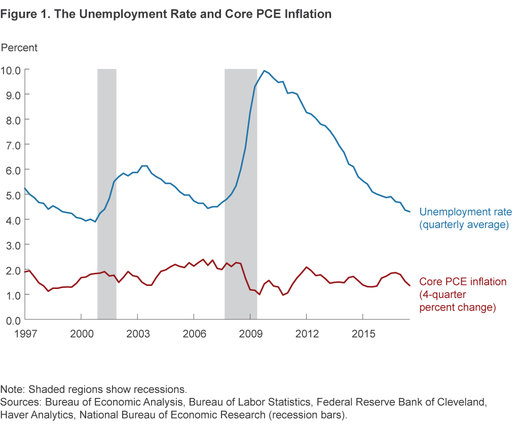
Finally, for the comparison point with the past, we use 1999:Q3. In selecting the comparison point, we sought out a time in which economic conditions bore similarities to today’s and forces that have been proposed as weighing on inflation—such as internet commerce and globalization—were arguably less important than they are today. Regarding the latter forces, the internet as an online marketplace was in its early stages in the late 1990s, and China had not yet entered the World Trade Organization. In terms of economic conditions, core PCE inflation was running below 2 percent in the late 1990s, while the unemployment rate was relatively low and declining (figure 1). In particular, the unemployment rate averaged 4.2 percent in 1999:Q3 while trailing four-quarter core PCE inflation was 1.3 percent; for comparison, the unemployment rate averaged 4.3 percent in 2017:Q3, and trailing four-quarter core PCE inflation was 1.3 percent.

Inflation: Still Partying Like It’s 1999?
A key benefit of the TVP-SV framework is that we can capture changes in inflation dynamics—even very recent changes that might only have occurred near the end of our estimation sample.5 These changes can take on a variety of forms, including changes in the persistence of our variables of interest; changes in the relationship between core inflation and the unemployment rate—that is, the slope of the Phillips curve; and changes in the model’s estimates of where the economy is likely to go in the long run.6 To see how the economy has changed since the late 1990s, we estimate the model twice, once using data through 1999:Q3 to capturecirca 1999 inflation dynamics and then a second time using data through 2017:Q3 to capture circa 2017 inflation dynamics.7
Table 1 reports key statistics from the two estimations. While the persistence of the unemployment rate is similar across the two periods, core inflation has become less persistent: The sum of the lagged inflation coefficients has decreased from 0.98 in the 1999:Q3 estimation to 0.87 in the 2017:Q3 estimation. The slope of the Phillips curve is just a little bit flatter in the later estimation: The unemployment rate has a slightly smaller influence on inflation circa 2017 than it did circa 1999, though the influence of the unemployment rate on inflation was already small in the late 1990s. But in the longer run, the two estimations expect the economy to converge to nearly identical places. Whether estimating using data through 1999 or 2017, the model calls for inflation to converge to 2 percent, while the unemployment rate converges to 4.3 percent when estimating through 1999 and 4.4 percent when estimating through 2017.8 So in both cases, the forces keeping inflation below 2 percent ultimately are viewed as transitory.
Table 1. Key Statistics from the Estimations
| 1999:Q3 estimation | 2017:Q3 estimation | |
|---|---|---|
| Inflation persistence | 0.98 | 0.87 |
| Unemployment persistence | 0.95 | 0.96 |
| Phillips curve slope | −0.07 | −0.06 |
| Long-run inflation | 2.0 | 2.0 |
| Long-run unemployment rate | 4.3 | 4.4 |
Source: Authors’ calculations.
Notes: Persistence and slope estimates are based on posterior mean parameter estimates. Long-run estimates are median forecast values after 10 years.
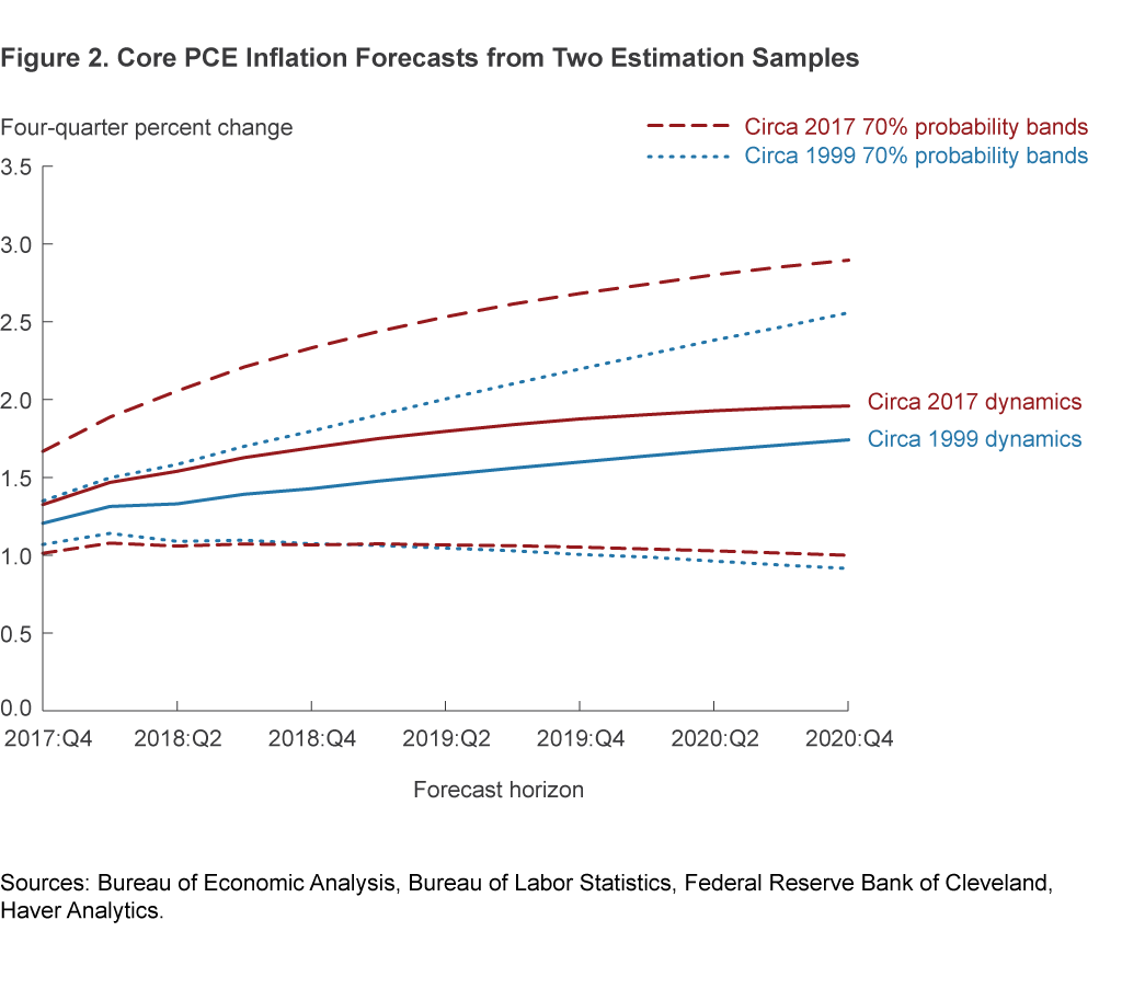
Using the recent data on core PCE inflation and the unemployment rate as a starting point, we take the estimated parameters based on the samples ending in 1999 and 2017 and produce two sets of forecasts, one based on circa 1999 inflation dynamics and another based on circa 2017 inflation dynamics. Figure 2 shows the inflation forecasts.9 The solid lines show the respective point forecasts, or most likely paths, from the two estimations. The corresponding dashed lines show the 70 percent probability bands around each point forecast; that is, they show the range of future inflation outcomes that the models expect will occur 70 percent of the time, with inflation expected to fall outside the bands 30 percent of the time. We make two observations.

First, we view the point forecasts for core PCE inflation as generally similar: Based on the inflation dynamics from either estimation period, the most likely path for inflation is a rising trajectory over the forecast horizon back toward 2 percent. If anything, the inflation projection based on circa 2017 dynamics is firmer than the projection based on circa 1999 dynamics. This finding comes largely from the fact that inflation is currently less inertial recently than it had been, a situation which allows inflation to return to its longer-run level more quickly in the recent period than it would have in the late 1990s. In both cases, the low level of the unemployment rate—which is below its longer-run level—is putting upward pressure on inflation via Phillips curve effects, but the strength of this effect is quantitatively similar for both forecasts. These results are at odds with the conjecture that growing forces—such as rising pressures from ongoing globalization and increased price competition from the internet—are depressing inflation and will continue to do so going forward.10
Second, considerable uncertainty surrounds these projections, but there is more uncertainty surrounding the point forecasts of inflation now than in the late 1990s. The differences in uncertainty are illustrated in the figure, because while the lower ends of the 70 percent probability bands are essentially identical across the two estimation periods, the upper bands are higher in the circa 2017 case than in the circa 1999 case. We find similar results for the unemployment rate, for which the 70 percent probability band is wider in the circa 2017 forecasts compared with that of the circa 1999 forecasts. The changing width of these probability bands is consistent with an economy that is now subject to larger shocks and a looser relationship between inflation and unemployment than in the past.
Given that the forecasts call for a firming of inflation, what actually occurred after 1999, when core PCE inflation and the unemployment rate were both near current levels? A common saying in the financial services industry is that past performance is no guarantee of future results—and that, in this case, may turn out to be a good thing. As figure 1 shows, core PCE inflation began to pick up in 2000 and was arguably headed back toward 2 percent—that is, until the unemployment rate rose with the 2001 recession and core inflation drifted back down. As the economy recovered, core PCE inflation did eventually make it to 2 percent, but not until 2004:Q4.
Conclusion
In this Commentary we use a flexible statistical model that can capture potential variation in inflation dynamics over time. We show that inflation forecasts based on inflation dynamics in two time periods, one in the late 1990s and another one in 2017, would both put inflation on a rising trajectory back toward 2 percent, with the forecast based on recent data suggesting the rise will be faster than would have been suggested by the late 1990s data. But we also document greater uncertainty around the more recent forecast path, consistent with an economy that is now subject to larger shocks and a looser relationship between inflation and unemployment than in the past.
Footnotes
- For example, Brainard (2017) notes that inflation expectations may have drifted down since before the crisis, thereby making it more difficult for inflation to rise to 2 percent. See Yellen (2017a) for a summary of the factors affecting inflation and some potential factors that may be contributing to changes in inflation dynamics. Return to 1
- The forecasting literature is generally critical of using Phillips curves to forecast inflation out of sample; see, e.g., Atkeson and Ohanian (2001), Stock and Watson (2007), Faust and Wright (2013), and Dotsey et al. (2017). But our approach does not rely on a Phillips curve, per se; for example, the inflation rate is not a function of the unemployment gap, and we omit forward-looking measures of inflation expectations that are part of the canonical New Keynesian Phillips curve (see, e.g., Coibion and Gorodnichenko 2015). Furthermore, D’Agostino et al. (2013) show that allowing for time-varying parameters and stochastic volatility, as we do, generally tends to improve inflation forecast accuracy. Return to 2
- As discussed in Knotek et al. (2015), the size of realized shocks in most macroeconomic models can vary over time, but the shocks are assumed to be drawn from a distribution with a standard deviation that is fixed. Models with stochastic volatility allow the standard deviation of the size of the shocks to change over time. Intuitively, stochastic volatility allows models to rapidly capture the changing size of the shocks hitting the economy. Return to 3
- We use Bayesian methods to estimate the model. Because estimation of TVP-SV models is computationally intensive and time-consuming, we incorporate two lags of each variable. Return to 4
- Compared with Primiceri (2005), we give the benefit of the doubt to potential time variation in our parameters by loosening the hyperparameters to k(Q)=0.08 and k(S)=0.5; otherwise, we largely follow Primiceri (2005), including using the first 40 observations as a training sample for setting the values of the prior distributions. We estimate the model beginning in 1969:Q2 and ending in either 1999:Q3 or 2017:Q3; in both cases, the training sample is from 1959:Q2 through 1969:Q1. The results are qualitatively similar using the same prior settings as in Primiceri (2005). Return to 5
- We measure the slope of our Phillips curve by summing the coefficients on the lagged unemployment rate variables in the core PCE inflation equation evaluated at the posterior mean of the parameter estimates. We measure persistence by summing the coefficients on their own lagged terms in each equation evaluated at the posterior mean of the parameter estimates. Return to 6
- In this way, we are using the same methodology to capture time variation through 1999:Q3 and through 2017:Q3, rather than estimating the model a single time through 2017:Q3 and then examining the estimated parameters in 1999:Q3. This latter single-estimation approach produces smaller differences between the two periods than what we document. Return to 7
- Because complete convergence can be extremely slow for persistent series, we measure the long run based on the median point forecasts after 10 years. The implied steady states based on the posterior mean of the parameter estimates are similar. Judgmentally, the longer-run estimates of the unemployment rate may appear a little low; for comparison, the range of longer-run estimates for the unemployment rate in the Federal Open Market Committee’s September Summary of Economic Projections was 4.5 percent to 5.0 percent, and the Congressional Budget Office’s June 2017 estimate of the long-term unemployment rate was 4.7 percent. But our estimates may not be completely implausible; e.g., Aaronson et al. (2015) estimate that changing demographics could push the natural rate of unemployment down to 3.9 percent by 2020. Return to 8
- While we do not show the forecasts for the unemployment rate, they are quite similar to each other: In both cases, the unemployment rate falls below 4 percent as of the first quarter of 2019. Thereafter, it drifts down very slowly in the circa 1999 case, while it starts to drift up very slowly in the circa 2017 case. Using relative entropy to impose the same path for the unemployment rate produces little change to the inflation forecasts we show. Return to 9
- Other analyses come to a similar conclusion; see, e.g., Mericle (2017) and Bianchi and Civelli (2015). Return to 10
References
- Aaronson, Daniel, Luojia Hu, Arian Seifoddini, and Daniel G. Sullivan. 2015. “Changing Labor Force Composition and the Natural Rate of Unemployment.” Federal Reserve Bank of Chicago, Chicago Fed Letter, Number 338.
- Atkeson, Andrew, and Lee E. Ohanian. 2001. “Are Phillips Curves Useful for Forecasting Inflation?” Federal Reserve Bank of Minneapolis, Quarterly Review, Winter: 2–11.
- Bianchi, Francesco, and Andrea Civelli. 2015. “Globalization and Inflation: Evidence from a Time Varying VAR.” Review of Economic Dynamics, 18(2): 406–433.
- Brainard, Lael. 2017. “Understanding the Disconnect between Employment and Inflation with a Low Neutral Rate.” Speech at the Economic Club of New York, New York, New York (September 5).
- Cogley, Timothy, and Thomas J. Sargent. 2005. “Drifts and Volatilities: Monetary Policies and Outcomes in the Post-WWII U.S.” Review of Economic Dynamics, 8(2): 262–302.
- Coibion, Olivier, and Yuriy Gorodnichenko. 2015. “Is the Phillips Curve Alive and Well After All? Inflation Expectations and the Missing Disinflation.” American Economic Journal: Macroeconomics, 7(1): 197–232.
- D’Agostino, Antonello, Luca Gambetti, and Domenico Giannone. 2013. “Macroeconomic Forecasting and Structural Change.” Journal of Applied Econometrics, 28(1): 82–101.
- Dotsey, Michael, Shigeru Fujita, and Tom Stark. 2017. “Do Phillips Curves Conditionally Help to Forecast Inflation?” Federal Reserve Bank of Philadelphia, Working Paper no. 17-26.
- Faust, Jon, and Jonathan H. Wright. 2013. “Forecasting Inflation.” In Graham Elliott and Allan Timmermann, eds., Handbook of Economic Forecasting, Volume 2, Elsevier: North Holland.
- Knotek, Edward II, Saeed Zaman, and Todd E. Clark. 2015. “Measuring Inflation Forecast Uncertainty.” Federal Reserve Bank of Cleveland, Economic Commentary, no. 2015-03.
- Mericle, David. 2017. “U.S. Daily: The Internet and Inflation: How Big Is the Amazon Effect?” Goldman Sachs Economics Research (August 2).
- Primiceri, Giorgio E. 2005. “Time Varying Structural Vector Autoregressions and Monetary Policy.” Review of Economic Studies, 72(3): 821–852.
- Stock, James H., and Mark W. Watson. 2007. “Why Has Inflation Become Harder to Forecast?” Journal of Money, Credit, and Banking, 39(S1): 3–33.
- Yellen, Janet L. 2017a. “Inflation, Uncertainty, and Monetary Policy” Speech at the “Prospects for Growth: Reassessing the Fundamentals.” 59th Annual Meeting of the National Association for Business Economics, Cleveland, Ohio (September 26).
- Yellen, Janet L. 2017b. “Transcript of Chair Yellen’s Press Conference” (September 20).
Suggested Citation
Knotek, Edward S., II, and Saeed Zaman. 2017. “Have Inflation Dynamics Changed?” Federal Reserve Bank of Cleveland, Economic Commentary 2017-21. https://doi.org/10.26509/frbc-ec-201721
This work by Federal Reserve Bank of Cleveland is licensed under Creative Commons Attribution-NonCommercial 4.0 International


