

- Share
Behavior of a New Median PCE Measure: A Tale of Tails
We introduce two new measures of trend inflation, a median PCE inflation rate and a median PCE excluding OER inflation rate, and investigate their performance. Our analysis indicates that both perform comparably to other simple trend inflation estimators such as the trimmed-mean PCE. Furthermore, we find that the performance of the median PCE is related to skewness in the distribution of cross-sectional growth rates across categories in the PCE, and our results suggest that the Bowley skewness statistic may be useful in forecasting.


The views authors express in Economic Commentary are theirs and not necessarily those of the Federal Reserve Bank of Cleveland or the Board of Governors of the Federal Reserve System. The series editor is Tasia Hane. This paper and its data are subject to revision; please visit clevelandfed.org for updates.
Revised on 8/21/2019 to correct the number of PCE components used and on 7/31/2019 to correct an error in the construction of figure 2 and to update the associated discussion.
Inflation refers to the common movement of prices in the economy, specifically the rate at which prices are generally rising or falling. In any given month, however, prices do not move in lockstep, as some prices rise rapidly, others rise slowly, and others fall. This variation in price movements can cause the average price level to bounce around significantly. When incoming price data feature a significant jump in the average, policymakers must deduce whether that jump represents the beginning of a sustained movement or whether it is transitory.
This is not a new problem, and a number of alternative approaches are used to estimate the trend in inflation. Some of these approaches are complex and require a deep knowledge of statistics to understand, while others are simpler and more transparent. In this Commentary, we introduce two simple measures of the trend in inflation that are based on the price index for personal consumption expenditures (PCE). The first is a median PCE inflation rate, and the second is a median PCE inflation rate excluding owners’ equivalent rent (commonly referred to as OER). We compare the performance of these two measures against two other simple measures that are currently produced and discussed (core PCE and the Dallas Fed trimmed-mean PCE).1 We highlight two main findings. First, both our median PCE inflation measure and our median PCE excluding OER inflation measure are useful indicators of the trend in inflation. Second, their performance relative to the other simple measures worsened after the Great Recession, and this worsening performance is related to the changing cross-sectional asymmetry of the growth rates of the components of PCE inflation.
The Problem of Tail Sensitivity
Price indexes are constructed in two stages. In the first stage, average price changes for numerous categories of goods and services are computed. For example, in a given month, the average price change in women’s shoes might be 3 percent, and the average price change in rent might be 2 percent.2 In the second stage, overall inflation is estimated as a weighted average over the growth rates of all of these categories or “components.” The weights are proportional to the expenditure shares of the average consumer for each of the components.
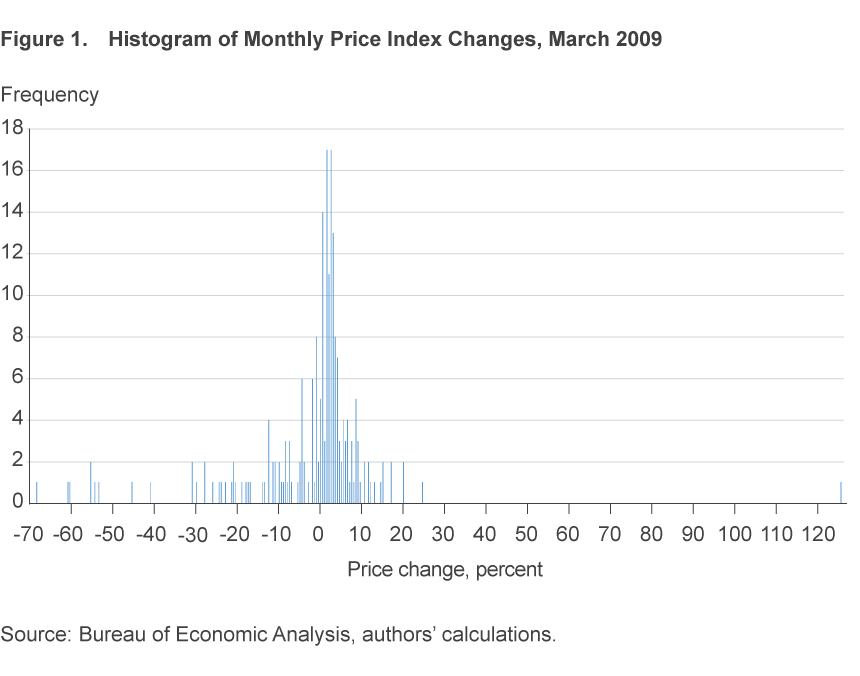
The PCE price index is constructed by the Bureau of Economic Analysis (BEA) as a weighted average of the price movements of 201 categories of goods and services each month.3 In a typical month most of the categories experience growth in the −3 percent to +6 percent range, but some categories—categories in the “tails of the distribution”—experience price changes that are much larger, such as −40 percent or +90 percent. To illustrate, figure 1 depicts a histogram of the growth rates of the 201 categories in March 2009. In that month, fuel oil dropped nearly 70 percent in price, with many other categories dropping in price by 20 percent or more, while tobacco had the most extreme price change, increasing by more than 125 percent.
Because the PCE index is constructed as a weighted average, it is sensitive to extreme observations. Movements in the tails can (and often do) drive the total, or “headline,” PCE index. This means that the average can be far from representative of the price changes in the middle of the distribution in a given month. For example, in March of 2009, the average price change was −1.0 percent, and the median price change (the price change in the middle of the distribution) was +1.9 percent. Energy prices fell about 36 percent during the month. But suppose that they had fallen by 72 percent instead. In that case, the average price change for March would have been −2.1 percent while the median would have been unaffected.
The sensitivity of headline PCE to large one-off movements in the tail of the price change distribution introduces volatility in the index that can make it difficult to discern the overall trend in prices. This is a problem for policymakers who wish to use headline PCE as a measure of the trend in inflation.
Simple Estimates of Trend Inflation
Because of the average’s sensitivity to the tail, a number of measures have been developed to get a more accurate gauge of the inflation trend. The simple trend measures considered in this Commentary all start from the monthly distribution of price changes like the one in figure 1, but then these trend measures differ in one of two ways: how they treat the tails, and whether or not they automatically exclude particular categories.
Core PCE inflation is one of the simplest and oldest measures of trend inflation. It excludes food and energy prices—whether or not these categories end up in the tails of the monthly distribution—and averages the movements of the rest. The rationale for developing this index was that food and energy price movements tend to be volatile and are often in the tails, as indeed they were in March 2009.
Trimmed-mean PCE (Dolmas, 2005) is calculated by the Federal Reserve Bank of Dallas. The Dallas Fed chops off the upper and lower tails of the price-change distribution—in particular, it drops the bottom 24 percent and the top31 percent of categories in any given month—and then takes the average of the remaining categories. At first glance, it may seem strange that a larger percentage is dropped from the upper tail than the lower tail; however, it follows from the asymmetry of the monthly price distribution.
Note that the distribution in figure 1 is not symmetric. There are extreme observations on both sides of the average. If we compute the Bowley sample skewness statistic, an estimator of skewness that is designed to be insensitive to extreme observations, we learn that the distribution in figure 1 is negatively skewed.4 Such negative skewness is fairly typical; since 1983, the cross-sectional distribution of the components of PCE inflation has been negatively skewed 60 percent of the time. When a sample is drawn from a negatively skewed distribution, the sample median will usually be greater than the sample mean. For the same reason, a symmetrically trimmed mean will have the same property once the trimming percentage becomes large enough. For instance, if we trim just the top 20 and bottom 20 categories from the March 2009 distribution, the resulting trimmed mean is −0.32, well above the sample mean. Intuitively, this symmetrically trimmed mean is removing too much of the influence of the lower tail, a lower tail which strongly influences the sample mean. The trimmed-mean PCE inflation measure trims a larger percentage from the upper tail than it does from the lower tail in order to correct for this bias.
Median PCE inflation is a measure we calculate by taking the weighted median of price changes among the full set of 201 price categories published by the BEA. By constructing our measure at the finest level of disaggregation available, we get the most accurate calculation of the median price change and reduce the volatility of our measure.
Why is a median useful? The rationale for the median starts with the fact that core PCE inflation will be volatile on occasion because categories other than food and energy can end up in the tails. A median is insensitive to extreme observations in the tails, regardless of the category. Research done at the Federal Reserve Bank of Cleveland on the consumer price index (CPI) in the early 1990s (e.g., Bryan and Pike, 1991, and Bryan and Cecchetti, 1993) indicated that a better trend inflation estimate might be the median price change among the categories. Other research has shown that the median CPI is useful in forecasting CPI inflation (see, e.g., Meyer and Zaman, 2018; Meyer, Venkatu, and Zaman, 2013). We investigate whether a median PCE will be similarly useful for assessing the trend in PCE inflation.
Median PCE excluding OER inflation is a measure we calculate by removing the two categories in the PCE index corresponding to owners’ equivalent rent (OER), leaving 199 categories, and then identifying the median price change. We investigate this second trend measure for two reasons. First, OER has a relatively large weight in the PCE price index, which may mean that it is frequently the weighted median category; previous work (Bednar and Knotek, 2014; Bednar and Clark, 2014) has investigated a similar index, median CPI excluding OER, and demonstrated the significant impact of OER on median CPI inflation. Second, there are still debates in the international statistics community as to the proper way to measure inflation for homeowners, and some countries simply omit OER.
Comparing the Simple Trend Measures
We evaluate the usefulness of the five indicators by comparing them on six key properties that are desirable in a simple trend inflation estimator:5
- Transparency of construction. A simple trend inflation estimator should be easily understood by the public and policymakers, and reasonably easy to replicate.
- Timeliness. A simple trend inflation estimator should be computable with little delay.
- Smoothness. A less volatile trend inflation estimator is preferable.
- Unbiasedness. A trend inflation estimator should result in the same average inflation rate as the underlying inflation series; or, if it is biased, its bias should be stable over time.
- Historical ability to track the underlying inflation trend. One should be able to verify that the estimator closely tracked a measure of the “true” trend in inflation.
- Forecasting ability. A trend inflation estimator should contain useful information for forecasting future headline PCE inflation.
How do the simple measures we consider here stack up on these criteria?
Transparency
Each of the indicators we examine is easily replicable. With the exception of the trimmed mean, each is easily explained. The trimmed mean is more challenging to explain to the public since one must discuss the rationale for its asymmetric trim.
Timeliness
All of the trend measures we consider are relatively simple to calculate and can be produced with minimal delay once the BEA releases the detailed data.
Smoothness
Regarding smoothness, the core PCE is far behind the other measures. Over the 1984–2016 time period, the standard deviation of 1-month changes in core PCE inflation is 1.45 percent. By contrast, over the same period, the standard deviation of trimmed-mean PCE inflation is 0.98 percent, the standard deviation of median PCE inflation is 1.02 percent, and the standard deviation of median PCE excluding OER inflation is 1.06 percent. For reference, the standard deviation of 1-month changes in headline PCE inflation is 2.29 percent.
Unbiasedness
Regarding bias, core PCE inflation initially appears to have a slight edge over the other trend estimates: Its bias over the entire 1979–2017 period is a mere +0.05 percentage points (ppt) on average. The bias of trimmed-mean PCE inflation is modest, roughly +0.13 ppt, while median PCE inflation and median PCE excluding OER inflation have upward biases of 0.52 ppt and 0.34 ppt, respectively.6 However, the apparent unbiasedness of core PCE inflation is illusory because its bias has experienced large fluctuations: For example, between 1995 and 2007, core PCE inflation was downward biased by 0.25 ppt, while between 1980 and 1985 it was upward biased by 0.3 ppt. In fact, computing the average bias over the following 10-year period for each month between January 1984 and July 2007 shows that the minimum bias attained by core PCE inflation was −0.49 ppt, the maximum bias was +0.35 ppt, and the standard deviation of its bias over that entire period is 0.31. The standard deviation of the bias of the other three trend estimates ranges between 0.13 and 0.17, indicating much more stability in bias over time. A trend estimate with stable bias is preferable to a trend estimate with bias that changes a lot over time, because it is easy to correct for the former. Thus, the unbiasedness property places core PCE inflation last.
Historical Ability to Track Inflation Trend
To assess the ability to track trend inflation, we first need to define the “true” trend in inflation. Previous research has mostly used a centered 36-month moving average (MA) as a measure of the “true” inflation trend (see, e.g., Bryan, Cecchetti, and Wiggins, 1997). Dolmas (2005) and Higgins and Verbrugge (2015) used several “true” inflation trend measures that are similar but which arguably have better properties. We use one from the latter study, a two-stage centered moving average, which we will refer to as the 2SMA trend. It moves similarly to a centered 36-month moving average but is superior to this in that it has no fluctuations that last less than 36 months.7 Owing to the bias noted above, we bias-correct each measure (against headline PCE inflation), including core PCE, prior to computing performance-comparison statistics. Bias correction is done using a rolling window over the previous 10 years, starting the comparison in January 1994 (so that the earliest data used are in January 1984).
Before turning to statistical results, we plot our simple, bias-corrected trend estimates (core PCE inflation, median PCE inflation, median PCE excluding OER inflation, and trimmed-mean PCE inflation) against the “true” inflation trend (as captured by the 2SMA trend) in figure 2. Except for the 2SMA trend, each is a 12-month change.
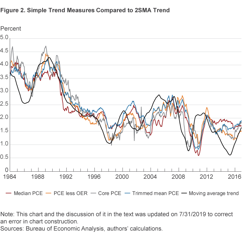
We highlight five findings from this graph. First, core PCE inflation stays closer to the moving-average trend than one might have expected, given its sensitivity to the tails. Second, the trend measures tend to move together, which suggests that they will have similar performance along many dimensions. Third, when median PCE excluding OER inflation departs from the others, such as in 1998–1999 and 2013–2015, it tends to run closer to the 2SMA trend, evidently driven by firm OER growth during those periods. But when median PCE inflation departs from the others, such as during 2003–2006 and 2012–2016, it tends to run farther from the 2SMA trend than the others. Fifth, we call attention to the joint behavior of the indexes from mid-2007 onward.
The 2SMA trend starts moving downward in mid-2007; since it is a centered moving average, it “knows ahead of time” the rapid decline in inflation that began at the start of the Great Recession.8 Conversely, the simple trend estimates start moving downward about 12 months later. This is because the other measures are lagging 12-month changes, so they will automatically lag turning points like this. The 2SMA trend begins to move upward in early 2009, and—temporarily—so does core PCE inflation.9 Meanwhile, the other measures do not begin to move upward until at least a year later. In addition, the 2SMA trend begins a long dip starting in 2013 that ends only in 2016; none of the simple trend estimates follows suit.
We provide a formal comparison of each simple measure of trend inflation with the “true” trend in inflation by looking at the square root of the mean squared errors (RMSEs) of core PCE, trimmed-mean PCE, and our two median PCE variants versus the 2SMA trend over the entire period. We look at both monthly and year-over-year movements in each candidate trend estimate. These RMSE results are reported in table 1. Regardless of the period, the trimmed-mean PCE is closest to the 2SMA on average when considering monthly changes, although the performance of median PCE excluding OER inflation is essentially as good. When considering 12-month changes, the median PCE excluding OER inflation rate runs closest to the 2SMA on average, followed by core PCE inflation. Broadly speaking, median PCE inflation does a slightly worse job at tracking headline inflation than the other simple trend measures by the RMSE criterion.
| Inflation measure | RMSE vs. 2SMA | |||
|---|---|---|---|---|
| 1984–2016 | 1984–2007:M6 | 2007:M7–2016 | ||
| Monthly | Core PCE | 1.14 | 1.27 | 0.91 |
| Trimmed-mean PCE | 0.68 | 0.63 | 0.73 | |
| Median PCE | 0.81 | 0.76 | 0.85 | |
| Median PCE excluding OER | 0.68 | 0.64 | 0.73 | |
| Year-over-year | Core PCE | 0.50 | 0.42 | 0.58 |
| Trimmed-mean PCE | 0.55 | 0.46 | 0.65 | |
| Median PCE | 0.64 | 0.54 | 0.75 | |
| Median PCE excluding OER | 0.43 | 0.34 | 0.53 | |
Note: In this table, we report the root mean squared error of each simple trend inflation indicator against a two-stage moving average of headline PCE inflation, which we are using to approximate the “true” trend in inflation. We report this for the full sample, and for two subsamples; and we report this at both the monthly frequency and at the year-over-year frequency.
Sources: Bureau of Economic Analysis, authors’ calculations.
Forecasting Ability
Finally, we examine forecasting ability by means of the following exercise. Following Blinder and Reis (2005) and Crone, Khettry, Mester, and Novak (2013), we run rolling-window regressions to predict-out-of-sample headline PCE inflation between today (t) and a given time in the future (h), either 6 months, 12 months, 24 months, or 36 months ahead. Each of these four headline inflation measures represents the annualized rate of inflation between t and t+h. For each horizon h, we use 120 months of data, with the first forecast starting in 1997:M1 (so that the earliest data used, for the 36-month horizon forecast, are 1984:M1) and the last forecast starting in 2013:M12 (so that the 36-month horizon ends in 2016:M12).10 The sole predictors are a constant term and the 12-month change in the trend inflation measure, which we denote xt−12,t.
πt,t+h = β0 + β1 xt−12,t + εt+h
Note that the inclusion of a constant term (β0) in these regressions helps to correct for the bias we documented earlier that is present in all of the trend measures. We compute the root mean squared forecast errors (RMSFEs) to determine whether a given simple trend measure improves or degrades forecast accuracy and use the Diebold-Mariano forecast test to determine whether a change in forecast accuracy is statistically significant. In table 2, we denote results that are statistically significant at the 10 percent, 5 percent, and 1 percent level by *, **, and *** respectively. (If forecast accuracy is worse, we use italics.) For comparison, we also include forecasting results from an exercise that uses headline PCE inflation over the previous 12 months to predict future headline PCE inflation.
| 1984–2007:6 | 2007:7–2016 | |||||||
|---|---|---|---|---|---|---|---|---|
| 6-month | 12-month | 24-month | 36-month | 6-month | 12-month | 24-month | 36-month | |
| PCE | 1.01 | 0.97 | 0.88 | 0.69 | 2.02 | 1.42 | 0.90 | 0.78 |
| Core PCE | 1.01 | 0.95 | 0.86 | 0.68 | 1.95*** | 1.29*** | 0.85*** | 0.75*** |
| Trimmed-mean PCE | 1.04 | 0.98 | 0.85 | 0.64* | 2.06 | 1.33*** | 0.97 | 0.95 |
| Median PCE | 1.04 | 0.96 | 0.76*** | 0.61*** | 2.02 | 1.28*** | 1.01 | 1.04 |
| Median excluding OER | 0.99* | 0.94** | 0.83*** | 0.62*** | 2.06 | 1.38 | 0.98 | 0.92 |
Notes: The reported RMSFEs indicate forecast accuracy of the simple trend measure relative to headline PCE. Italics indicate worse forecast accuracy. * indicates significance at the 10 percent level; ** significance at the 5 percent level; and *** significance at the 1 percent level.
Sources: Bureau of Economic Analysis, authors’ calculations.
In preliminary results, we found that forecast accuracy changed markedly starting in mid-2007. Thus, for brevity, we present forecasting results over the period 1984–2007:M6 and over the period 2007:M7–2016, but omit those for the full sample.
In the early period, at the 6-month horizon, only one of the simple trend estimators—median PCE excluding OER inflation—has historically produced improved forecasts over simply using headline inflation, but the improvement is marginal. Most of the other simple trend indicators have produced less accurate forecasts. At the 12-month horizon, only median PCE excluding OER inflation has produced significantly better predictions (significant at the 5 percent level). However, at the 24-month and 36-month horizons, things are different. At those horizons, the historical forecasts from median PCE inflation and median PCE excluding OER inflation have been more accurate than those from the headline PCE, with median PCE inflation holding an advantage over the other three trend measures. From the perspective of mid-2007, it would have been reasonable to conclude that one should use median PCE inflation for forecasts at these horizons.
In the late period, the early-period forecasting results are almost flipped. Over the later period, all of the simple trend estimators except median PCE excluding OER inflation have generated significant gains in forecast accuracy at the 12-month horizon. At other horizons, it is core PCE inflation alone—which is the trend indicator that was of no help in the earlier period—that provides statistically significant forecast gains.
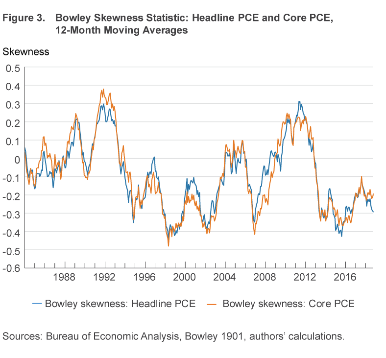
To explain these results, we look at the tails of the distribution of price changes among the components of inflation. In figure 3, we plot a 12-month moving average of the Bowley skewness statistic for headline PCE inflation and core PCE inflation for the period 1984–2016. During the four periods when skewness became deeply negative—1997–1999, 2001–2002, 2006–2007, and 2013–2016—the median PCE inflation rate was notably above the 2SMA trend (see figure 2). Conversely, when skewness was highly positive, from mid-2009–2012, the median PCE inflation rate was notably below the 2SMA trend. Median PCE excluding OER inflation was less subject to upward bias during these periods, presumably because OER (the omitted category) was well above average during those periods. Core PCE inflation, meanwhile, was driven by the tails during these episodes, and it overshot the 2SMA trend. These results suggest that the Bowley skewness statistic may be useful in forecasting; its inclusion in the forecasting model will provide a way to “correct” the median during periods of strong skewness, which are the periods during which the median is farthest from the mean. Furthermore, our results suggest that it may be worth considering other trend inflation measures as well, because strong skewness in the underlying distribution can imply that other estimators provide better estimates of the mean of the distribution than does the sample average.11
Our reading of this statistical evidence is that while most of the simple trend estimates perform well along various dimensions, none of the simple trend measures dominates the others along all dimensions. Trimmed-mean PCE inflation and median PCE inflation, estimators which use reliable approaches to estimate the broader trend of price movements, perform well except when the cross-sectional distribution of price changes is strongly skewed. The performance of median PCE excluding OER inflation appears quite good (especially as a read on current trend inflation) even though this measure is built upon a foundation that omits an inflation category, OER, that is significant in headline PCE. Core PCE inflation has a decidedly mixed performance. During the post-2007 period, it produced superior forecasts of headline PCE inflation. But it is worth emphasizing two drawbacks: the significant bias of this measure over long periods of time and the notable volatility of the bias. This measure’s forecasting advantage over the post-2007 period follows from the fact that the measure was driven by the tails of the distribution in a manner similar to headline PCE during this period.
Conclusion
Divining the trend in inflation is a constant challenge for economists. In this Commentary, we introduced two new measures of trend inflation, a median PCE inflation rate and a median PCE excluding OER inflation rate, and investigated their performance. Our analysis indicates that both perform comparably to other simple trend inflation estimators such as the trimmed-mean PCE. Furthermore, as performance of the median PCE is related to skewness in the distribution of cross-sectional growth rates across categories in the PCE, our results suggest that the Bowley skewness statistic may be useful in forecasting.
Footnotes
- The Federal Reserve Bank of San Francisco previously published a median PCE as part of its suite of PCE dispersion measures. Relative to our median PCE measures, the San Francisco Fed’s median used a notably coarser grouping of the PCE items. Return to 1
- In this Commentary, we report inflation as month-over-month annualized percent changes because we typically think of inflation in terms of annual rates. Return to 2
- The number of categories has increased over time. The price movement of a category, such as shoes and footwear, is in turn the average price movement of a large number of prices of very specific items. Return to 3
- Dolmas (2005) finds negative skewness with three alternative robust skewness estimators, of which, the Bowley (1901) skewness statistic is one. Note that skewness in the distribution of price changes across categories has no necessary relationship to skewness of price changes within a particular category. Return to 4
- For more discussion of these properties see Wynne (2008), Clark (2001), Rich and Steindel (2007), Silver (2007), or Higgins and Verbrugge (2015). Return to 5
- In constructing the trimmed-mean PCE inflation measure, different percentages were allowed to be trimmed from the top and the bottom of the distribution in order to minimize its bias; hence, its performance along this dimension is not surprising. Conversely, by construction a median trims exactly the same percentage of observations from the top and the bottom of the distribution. Return to 6
- This moving average is constructed by first applying a 24-month (centered) moving average to headline PCE inflation, followed by a 12-month (centered) moving average. For details on the comparison, see Higgins and Verbrugge (2015). Return to 7
- See Stock and Watson (2010) and Ashley and Verbrugge (2019), who demonstrate that such deceleration at the onset of recessions constitutes the predominant Phillips curve relationship. Return to 8
- Ashley and Verbrugge (2019) note that the abrupt rebound in core PCE inflation in 2009 was driven by sharp upward movements in prices that were not market-determined; the market-determined prices in core PCE moved similarly to the trimmed-mean PCE. Headline PCE inflation was, of course, also influenced by these sharp movements in non-market-determined prices. Return to 9
- Crone et al. (2013) use 101 months of data for their forecast comparison exercise. Return to 10
- For instance, statistical theory indicates winsorizing a sample can be useful, and that optimal trimming can depend upon the degree and nature of the asymmetry (see, e.g., Jureckova, Koenker, and Welsh 1994 or Olive 2008). Return to 11
References
- Ashley, Richard, and Randal Verbrugge. 2019. “Variation in the Phillips Curve Relation across Three Phases of the Business Cycle.” Federal Reserve Bank of Cleveland Working Paper, No. 19-09.
- Bednar, Bill, and Edward S. Knotek II. 2014. “What’s Up in Inflation? Shelter and OER.” Federal Reserve Bank of Cleveland, Economic Trends, 02.21.14.
- Bednar, Bill, and Todd E. Clark. 2014. “Methods for Evaluating Recent Trend Inflation.” Federal Reserve Bank of Cleveland, Economic Trends, 03.28.14.
- Blinder, Alan S., and Ricardo Reis. 2005. “Understanding the Greenspan Standard.” In The Greenspan Era: Lessons for the Future. A Symposium Sponsored by the Federal Reserve Bank of Kansas City, Jackson Hole, Wyoming, August 25–27.
- Bowley, Arthur Lyon. 1901. Elements of Statistics. P.S. King & Son, London.
- Bryan, Michael F., and Christopher J. Pike. 1991. “Median Price Changes: An Alternative Approach to Measuring Current Monetary Inflation.” Federal Reserve Bank of Cleveland, Economic Commentary, 12.01.1991.
- Bryan, Michael F., and Stephen G. Cecchetti. 1993. “The Consumer Price Index as a Measure of Inflation.” Federal Reserve Bank of Cleveland, Economic Review, 4:15–24.
- Bryan, Michael F., Stephen G. Cecchetti, and Rodney L. Wiggins II. 1997. “Efficient Inflation Estimation.” NBER Working Paper, No. 6183.
- Clark, Todd E. 2001. “Comparing Measures of Core Inflation.” Federal Reserve Bank of Kansas City, Economic Review, 86(2): 5–31.
- Crone, Theodore M., N. Neil K. Khettry, Loretta J. Mester, and Jason A. Novak. 2013. “Core Measures of Inflation as Predictors of Total Inflation.” Journal of Money, Credit, and Banking, 45(2-3): 505–519.
- Dolmas, Jim. 2005. “Trimmed-Mean PCE Inflation.” Federal Reserve Bank of Dallas, Working Paper, No. 0506.
- Higgins, Amy, and Randal Verbrugge. 2015. “Is a Nonseasonally Adjusted Median CPI a Useful Signal of Trend Inflation?” Federal Reserve Bank of Cleveland, Economic Commentary, No. 2015-13.
- Jureckova, Jana, Roger W. Koenker, and A. H. Welsh. 1994. “Adaptive Choice of Trimming Proportions.” Annals of the Institute of Statistical Mathematics, 46: 737–755.
- Meyer, Brent H., Guhan Venkatu, and Saeed Zaman. 2013. “Forecasting Inflation? Target the Middle.” Federal Reserve Bank of Cleveland, Economic Commentary, No. 2013-05.
- Meyer, Brent H., and Saeed Zaman. 2018. “The Usefulness of the Median CPI in Bayesian VARs Used for Macroeconomic Forecasting and Policy.” Empirical Economics, forthcoming.
- Olive, David J. 2008. “Applied Robust Statistics.” Unpublished manuscript, Southern Illinois University.
- Rich, Robert, and Charles Steindel. 2007. “A Comparison of Measures of Core Inflation.” Federal Reserve Bank of New York, Economic Policy Review, (Dec): 19–38.
- Silver, Mick. 2007. “Core Inflation: Measurement and Statistical Issues in Choosing among Alternative Measures.” IMF Staff Papers, 54(1):163–190.
- Stock, James H., and Mark W. Watson. 2010. “Modeling Inflation after the Crisis.” National Bureau of Economic Research, Working Paper No. 16488.
Suggested Citation
Carroll, Daniel R., and Randal J. Verbrugge. 2019. “Behavior of a New Median PCE Measure: A Tale of Tails.” Federal Reserve Bank of Cleveland, Economic Commentary 2019-10. https://doi.org/10.26509/frbc-ec-201910
This work by Federal Reserve Bank of Cleveland is licensed under Creative Commons Attribution-NonCommercial 4.0 International

