

- Share
Lingering Residual Seasonality in GDP Growth
Measuring economic growth is complicated by seasonality, the regular fluctuation in economic activity that depends on the season of the year. The Bureau of Economic Analysis uses statistical techniques to remove seasonality from its estimates of GDP, and, in 2015, it took steps to improve the seasonal adjustment of data back to 2012. I show that residual seasonality in GDP growth remains even after these adjustments, has been a longer-term phenomenon, and is particularly noticeable in the 1990s. The size of this residual seasonality is economically meaningful and has the ability to change the interpretation of recent economic activity.

The views authors express in Economic Commentary are theirs and not necessarily those of the Federal Reserve Bank of Cleveland or the Board of Governors of the Federal Reserve System. The series editor is Tasia Hane. This paper and its data are subject to revision; please visit clevelandfed.org for updates.
Every quarter, the Bureau of Economic Analysis (BEA) releases estimates of gross domestic product (GDP), an indicator that is generally taken to be the broadest measure of the country’s economic activity. Because of its wide applicability, both policymakers and business economists closely follow the BEA’s estimates of GDP growth in order to monitor the pace of economic growth and watch for potential recessions.
However, tracking the health of the economy with GDP is complicated by seasonality, the regular fluctuation in economic activity that depends on the season of the year. This seasonal fluctuation partly depends on natural cycles. For example, new houses are most commonly started in the spring and built over the summer when the weather is the most accommodating. Seasonality also results from social customs. For example, end-of-year holidays, such as Christmas, generate increased gift-giving and consumer spending in the fourth quarter of the year.
Seasonality is large and makes assessing the state of the business cycle difficult.1 Thus, the BEA uses statistical techniques to remove seasonality from its estimates of GDP, and these estimates are commonly taken as reliable indicators of the health of the economy that are free of seasonality. However, economists have recently begun to ask if there is residual or leftover seasonality in GDP, and they have not reached an agreement. Rudebusch, Wilson, and Mahedy (2015) and Stark (2015) argue that residual seasonality does exist. However, Groen and Russo (2015) and Gilbert, Morin, Paciorek, and Sahm (2015) disagree.
In this Commentary, I revisit the question of whether the BEA’s estimates of GDP from 1985 to 2015 contain residual seasonality.2 I do so using new sophisticated statistical techniques that offer some advantages over those used in prior work on the subject. Specifically, these techniques work well when the data on the variable of interest display significant correlation across time. 3 Because of this attribute, assessments of residual seasonality based on these techniques might be more reliable than those based on older techniques. Moreover, by using statistical tools that differ from those used in previous studies, I can help determine which results from these studies are robust.
Using these techniques, I find residual seasonality. On average, first-quarter GDP growth from 1985 to 2015 has residual seasonality of annualized −0.8 percent. This residual seasonality is not driven by recent data and is particularly noticeable in the 1990s. During the same time period, second-quarter GDP growth has residual seasonality of annualized 0.6 percent on average. This has caused a regular bounce-back effect where GDP growth appears to slow in the first quarter of the year and speed back up in the second quarter of the year.
The residual seasonality is driven by residual seasonality in two components of GDP: private investment and government consumption and investment. Moreover, it is important to note that this residual seasonality is present even after new seasonal adjustments were introduced by the BEA in 2015. These findings show that residual seasonality in GDP growth continues to be a problem, and business economists and policymakers should take it into account when assessing the health of the economy. Further, because residual seasonality is present as far back as the 1990s, seasonal adjustments should be considered when using historical data for statistical models of forecasting or policy analysis.
A Description of the Methodology and Evidence ofResidual Seasonality
There are two important difficulties in trying to identify residual seasonality. The first is separating the business cycle from any seasonal component in the data. For example, GDP growth was −2.7 percent in the first quarter of 2008. Should this fall in GDP be taken as evidence of residual seasonality or attributed to the beginning of the Great Recession?4 The second difficulty is separating actual residual seasonality from coincidence. Much like it is possible for a fair coin to show heads for several flips in a row, it is possible for first-quarter GDP growth to be unusually low for several years in a row. For example, a string of winters that are more severe than usual can cause unusually low first-quarter GDP growth without residual seasonality being present. This is because seasonal adjustments only account for typical fluctuations in economic activity, and atypically severe winters would just be considered randomness in the data.
Given these difficulties, the methodology I use focuses on two tasks. The first is separating the business cycle from any potential seasonal component of GDP. The second is testing for long-run evidence of residual seasonality.
I model GDP growth as having three components: a business-cycle component (ct), a seasonal component (st), and an irregular component (it). These components sum to give GDP growth as follows:
yt = ct + st + it.
The business-cycle component includes fluctuations in GDP growth associated with recessions and recoveries as well the average level of GDP growth from 1985 to 2015. I define the seasonal component to be regular deviations from the business-cycle component that are associated with a given quarter of the year. Finally, the irregular component includes any fluctuations in GDP growth that cannot be attributed to the cyclical or seasonal components.5
With the above decomposition of GDP growth, I use a four-step procedure to test for residual seasonality.
In the first step, I take GDP growth from 1985 to 2015, estimate the business-cycle component, and subtract this component from overall growth. My approach to the estimation is to use a linear regression to account for the patterns in GDP growth that are associated with fluctuations lasting two years or more. Fluctuations lasting two years or more will include those associated with economic recessions and expansions. However, the two-year cutoff is long enough not to interfere with any potential seasonal pattern, which would last less than one year.
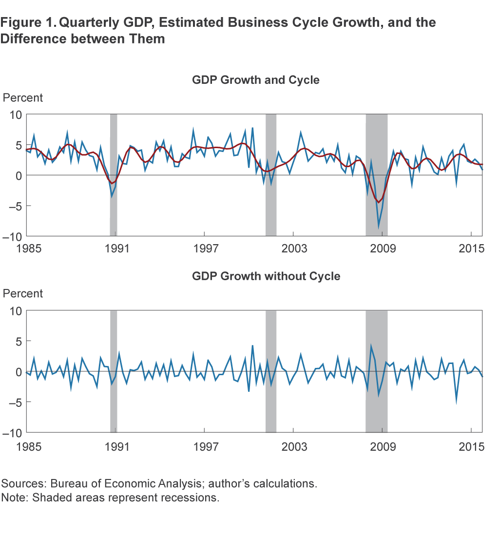
Figure 1 displays the estimated business cycle along with the quarterly estimates of GDP growth (panel A).6 We can see that the estimated cycle is a smoothed version of GDP growth, and it picks up much of the fluctuation in GDP growth around all three recessions in the sample. Panel B displays the difference between GDP growth and the estimated cycle. The data in this panel should be free of any influence from the business cycle, and visual inspection indicates that this is the case.
Figure 1. Quarterly GDP, Estimated Business Cycle Growth, and the Difference between Them
In the second step of the process for testing for residual seasonality, I collect the difference between GDP growth and its estimated business cycle, which is the data in panel B of figure 1, by quarter of the year. Then, in the third step, I calculate the average of the quarter-by-quarter differences between GDP growth and its cycle. Finally, in the fourth step, I produce confidence intervals for the averages from the third step using statistical techniques taken from Müller and Watson’s (2008, 2015) low-frequency econometrics. The intent of steps two through four is to check for regular deviations from the business cycle that are associated with a given quarter of the year.
Figure 2 summarizes the results of steps two through four. Each panel displays the results for a given quarter and shows the difference between GDP growth and the estimated business cycle for the quarter, the quarterly average, and the 95 percent confidence intervals around the averages. This figure shows that the first quarter has an average seasonaleffect of −0.8 percent. Further, because the confidence interval for this average is entirely below zero, this seasonal effect is statistically significant and indicates the existence of residual seasonality. Also notice that the residual seasonality in first-quarter GDP growth is not a recent phenomenon. The difference between GDP growth and the estimated business cycle for quarter 1 indicates that GDP growth was consistently below the business cycle throughout the 1990s.
Figure 2. Difference between GDP Growth and the Estimated Cycle by Quarter
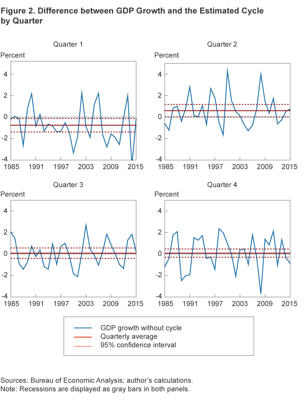
Another important result displayed in figure 2 is that the second quarter has an average seasonal effect of 0.6 percent. This seasonal effect is statistically significant and indicates the existence of residual seasonality in the second quarter of the year. Because any seasonal effect that might exist averages out over the course of the year, figure 2 indicates that the negative effect of seasonality on growth in the first quarter is almost entirely corrected in the second quarter. That is, GDP growth regularly bounces back in the second quarter after its first-quarter slump.
The final result from figure 2 is that the third and fourth quarters each have an average seasonal component of 0.1 percent. However, these averages are not statistically significant, indicating no residual seasonality in these quarters. These results are largely consistent with the findings of Rudebusch, Wilson, and Mahedy (2015) and Stark (2015). In particular, the size of the residual seasonality in the first and second quarters is similar to Stark’s findings. Further, Rudebusch, Wilson, and Mahedy also find low first-quarter GDP growth dating back to the 1990s.
In its 2015 annual revision to the GDP estimates, the BEA took steps to improve its seasonal adjustment of GDP components, including making seasonal adjustments to personal consumption expenditures, inventories, and government expenditures for defense (McCulla and Smith 2015). These adjustments went back to 2012 and are included in the data for this analysis. As shown in figure 2, residual seasonality in GDP growth remains even after these adjustments. This is largely due to the fact that the residual seasonality is present back to the 1990s, and the annual revision adjusts back to only 2012. Further, as McCulla and Smith show, first-quarter GDP growth remains lower than growth in the other quarters from 2012 to 2015, even after the revision.
The Source of Lingering Residual Seasonality
The BEA’s estimates of GDP come from four components: personal consumption, private investment, net exports, and government consumption and investment. Further, each of these components is also estimated from subcomponents. In this section, I test for residual seasonality in each of these components and their subcomponents by applying the same four-step process that I applied to GDP growth. The purpose of this exercise is to find the source of the residual seasonality in GDP growth.
Table 1 displays the average seasonal effect in percent for each component and subcomponent of GDP growth in each quarter of the year. Table 1 also indicates whether these seasonal effects are statistically significant at the 5 percent and 10 percent levels. The data to produce this table come from NIPA table 1.1.2, which gives the percent contribution to the percent change in GDP growth. Thus, the values for each subcomponent sum up to the value of the component aside from rounding error.
| Q1 | Q2 | Q3 | Q4 | ||
|---|---|---|---|---|---|
| GDP | −0.76** | 0.60** | 0.08 | 0.08 | |
| Consumption | −0.09 | −0.03 | 0.29 | −0.17 | |
| Durable goods | −0.06 | 0.01 | 0.26 | −0.21 | |
| Nondurable goods | −0.02 | −0.01 | −0.03 | 0.06 | |
| Services | −0.01 | −0.03 | 0.06* | −0.02 | |
| Private investment | −0.33** | 0.33** | −0.25 | 0.25 | |
| Nonresidential structures | −0.07 | 0.06 | 0.03 | −0.01 | |
| Nonresidential equipment | −0.03 | 0.07 | 0.07 | −0.10* | |
| Nonresidential intellectual property | −0.01 | −0.01 | 0.00 | 0.02 | |
| Residential investment | −0.02 | 0.09** | −0.03* | −0.04* | |
| Change in private inventories | −0.20 | 0.12 | −0.31** | 0.38* | |
| Net exports | −0.07 | −0.03 | −0.03 | 0.13 | |
| Exports | −0.22 | 0.11 | −0.06 | 0.17* | |
| Imports | 0.16 | −0.14 | 0.02 | −0.04 | |
| Government consumption and investment | −0.27** | 0.33** | 0.07 | −0.13 | |
| Federal: National defense | −0.26** | 0.28** | 0.14* | −0.16* | |
| Federal: Nondefense | 0.03 | −0.01 | −0.05 | 0.03 | |
| State and local | −0.03 | 0.06 | −0.03 | 0.00 | |
Note: One star indicates statistical significance at the 10 percent level, and two stars indicate statistical significance at the 5 percent level.
Sources: Bureau of Economic Analysis; author’s calculations.
Of the four major components of GDP, private investment and government consumption and investment contribute the most to the residual seasonality in total GDP growth in the first and second quarters. Consumption and private investment also have large values of residual seasonality in the third and fourth quarters. However, these values are not statistically significant and hence cannot be distinguished from just being noise in the data.
When looking at the subcomponents of government consumption and investment, national defense drives nearly all of the residual seasonality. Further, this residual seasonality in national defense is large, contributing about one-third of the first-quarter residual seasonality in GDP growth and about one-half of the second-quarter residual seasonality in GDP growth.
When looking at the subcomponents of private investment, it is not clear what is driving the residual seasonality. Change in private inventories has large residual seasonality, but this seasonality is only statistically significant in the third and fourth quarters. Residential investment also has residual seasonality, but it is quantitatively small. It may be the case that there is correlation in the seasonality of the subcomponents of private investment, and the correlation is driving the seasonality in total private investment. However, that correlation is not immediately clear from table 1.
My finding of residual seasonality in private investment and government consumption and investment is consistent with Stark (2015). However, Stark finds residual seasonality in exports and imports, which I do not find in this analysis.
Conclusions
This Commentary provides evidence of residual seasonality in GDP growth from 1985 to 2015. During this period, first-quarter GDP growth has residual seasonality of annualized −0.8 percent, and second-quarter GDP growth has residual seasonality of annualized 0.6 percent. This residual seasonality is driven by private investment and government consumption and investment. In particular, residual seasonality in national defense makes a large contribution to residual seasonality in total GDP growth.
The size of this residual seasonality is economically meaningful and has the ability to change the interpretation of recent economic activity. In the first and second quarters of 2016, the BEA estimates of GDP growth are 0.8 percent and 1.4 percent, respectively. This indicates slow but rising growth in the first half of 2016. However, after adjusting these numbers for the residual seasonality in GDP growth, they are 1.6 percent in the first quarter and 0.8 percent in the second quarter. The adjusted data still indicate a low level of growth; however, they now indicate that growth slowed in the first half of 2016, rather than rose, as indicated by data that do not undergo this second round of adjustment. This slowing in first-half growth is more consistent with other economic variables. For example, an alternative measure of GDP, called gross domestic income, had estimated growth of 0.8 percent and −0.2 percent in the first and second quarters of 2016, respectively.7 In addition, employment increased by 587,000 in the first quarter of 2016 but only by 439,000 in the second quarter.
While the BEA’s 2015 annual revision took steps to improve seasonal adjustment, those steps affected data back only to 2012. I show that residual seasonality in GDP growth has been a longer-term phenomenon and is particularly noticeable in the 1990s. Given that historical GDP data are often incorporated into statistical models of forecasting and policy analysis, users of these models should consider seasonally adjusting GDP growth before producing forecasts or analyzing economic policy.
Footnotes
- Barsky and Miron (1989) show that growth in real gross national product averaged −8.1 percent, 3.7 percent, −0.5 percent, and 4.9 percent in the first, second, third, and fourth quarters, respectively, from 1948 to 1985. Rudebusch, Wilson, and Mahedy (2015) show that growth in nominal gross domestic product averaged about −10 percent and 20 percent in the first and second quarters, respectively, from 2000 to 2006. Return
- Formally, I test the null hypothesis that no residual seasonality is present. Return
- In technical terms, consistent estimators of long-run variances, such as Newey and West (1987), can perform poorly for hypothesis testing when data are moderately correlated across time. This is particularly problematic for the analysis in this Commentary because I use estimates of long-run variances to construct confidence intervals for hypothesis testing. To get around this problem, I use the low-frequency econometrics of Müller and Watson (2008, 2015) to estimate long-run variances. Müller (2007) shows that long-run variance estimators of the type used in Müller and Watson (2008, 2015) maintain the targeted statistical size for moderately persistent data. Return
- Wright (2013) documents the difficulty in separating the business cycle from seasonal adjustments in employment data. Return
- This decomposition of GDP growth into three components parallels the decomposition used in the Census Bureau’s X-13 seasonal adjustment filter. The only difference is that I use the vocabulary “business-cycle” component in place of the Census’s “trend” component. Return
- GDP growth is from line 1 of national income and products account (NIPA) table 1.1.2. Return
- Using the methodology described in this Commentary, I find no residual seasonality in gross domestic income growth. Return
References
- Barsky, Robert B., and Jeffrey A. Miron, 1989. “The Seasonal Cycle and the Business Cycle,” Journal of Political Economy, 97(3): 503–534.
- Gilbert, Charles, Norman J. Morin, Andrew D. Paciorek, and Claudia R. Sahm, 2015. “Residual Seasonality in GDP,” Board of Governors of the Federal Reserve System, FEDS Notes, May 14.
- Groen, Jan, and Patrick Russo, 2015. “The Myth of First-Quarter Residual Seasonality,” Federal Reserve Bank of New York, Liberty Street Economics, June 8.
- McCulla, Stephanie H., and Shelly Smith, 2015. “Preview of the 2015 Annual Revision of the National Income and Product Accounts,” Bureau of Economic Analysis, Survey of Current Business, June.
- Müller, Ulrich K., 2007. “A Theory of Robust Long-Run Variance Estimation,” Journal of Econometrics, 141(2): 1331–1352.
- Müller, Ulrich K., and Mark W. Watson, 2008. “Testing Models of Low-Frequency Variability,” Econometrica, 76(5): 979–1016.
- Müller, Ulrich K., and Mark W. Watson, 2015. “Low-Frequency Econometrics,” NBER Working Paper, No. 21564.
- Newey, Whitney K., and Kenneth D. West, 1987. “A Simple, Positive Semi-Definite, Heteroskedasticity and Autocorrelation Consistent Covariance Matrix,” Econometrica, 55(3): 703–708.
- Rudebusch, Glenn D., Daniel Wilson, and Tim Mahedy, 2015. “The Puzzle of Weak First-Quarter GDP Growth,” Federal Reserve Bank of San Francisco, Economic Letter, 2015–16.
- Stark, Tom, 2015. “First Quarters in the National Income and Product Accounts,” Federal Reserve Bank of Philadelphia, Research Rap Special Report, May 14.
- Wright, Jonathan H., 2013. “Unseasonal Seasonals?” Brookings Papers on Economic Activity, Fall, 65–110.
Suggested Citation
Lunsford, Kurt G. 2017. “Lingering Residual Seasonality in GDP Growth.” Federal Reserve Bank of Cleveland, Economic Commentary 2017-06. https://doi.org/10.26509/frbc-ec-201706
This work by Federal Reserve Bank of Cleveland is licensed under Creative Commons Attribution-NonCommercial 4.0 International

