US Labor Market after COVID-19: An Interim Report

The 2020 pandemic recession was unique compared to previous recessions. First, as pointed out by Kouchekinia et al. (2020), the vast majority of layoffs during the pandemic have been temporary. Compared to permanent layoffs, temporary layoffs are short-lived and are more likely to end through a job recall. Second, unlike during the economic downturn triggered by the 1918–1920 H1N1 influenza pandemic, the number of deaths directly attributed to pandemic-related illness among the working-age (also known as “prime-age”) population has been relatively small. For example, prime-age individuals represented only 10.4 percent of COVID-19-related deaths during the current pandemic; during the 1918–1920 H1N1 influenza pandemic, prime-age individuals comprised 43.5 percent of pandemic-illness-related deaths. As a result, deaths by H1N1 in 1918–1920 represented a 0.9 percent decline in the prime-age population, compared to an 0.08 percent decline in the same population group in the case of COVID-19.² However, deaths are not the only component of a pandemic that may affect labor supply. Early retirements have also had an impact on the labor force participation rate, which remains 1 percentage point below its prepandemic level. These retirements, while allowing younger workers to move out of low-wage occupations, created a shortage of labor in some occupations (see Forsythe et al., 2022). Finally, the pandemic altered the productive process by changing working arrangements, a situation which makes past experiences less likely to be informative about where the economy is heading.

In this environment, a detailed comparison of the job market patterns before and after the COVID-19 pandemic will prove informative regarding what we might expect in the coming years. This Commentary is a first step in that direction. Using data from January 2019 through August 2022, we see changes in employment across space that indicate an uneven recovery. Without attributing causality, we find that denser metropolitan areas and those that imposed stricter measures to contain the spread of COVID-19 observed a slower recovery on employment levels and labor force participation. In contrast, there is limited evidence that changes in work arrangements, or remote work, impacted the distribution of economic activity across space.

An Uneven Recovery

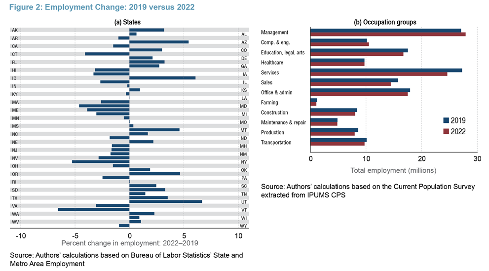
As we see in Figure 1, total employment is back to prepandemic levels. However, Figure 2a also depicts the significant variation across states. While Utah observed employment growth above 6 percent since 2019, Vermont remains 6.5 percent below its 2019 average employment.³ Similarly, while services and sales occupations are down 6 percent and 7 percent, respectively, since 2019, management and computer and engineering occupations are up 7 percent and 10 percent, respectively, as seen in Figure 2b.

We present some factors that may be correlated to this uneven recovery. Note that our analysis aims to highlight factors that may have played a role, but we are unable to attribute either causality or the mechanism through which such factors impact employment. In particular, measures taken to curb the effects of the pandemic may depend on information that is not available to researchers (an issue known as “omitted variable bias”). This lack of information may vary across space and thereby explain the variation observed across states. Second, the measures taken may have helped prevent a worse scenario than the one observed. Being unable to observe this “counterfactual scenario” (that is, what would have happened without the implemented measures) prevents us from attributing causality to the observed correlations. Nevertheless, the analysis presented in this Commentary is an important first step in highlighting factors that may have contributed to the ongoing recovery.

We focus on the harshness of the pandemic and the measures used to curb it while controlling for demographic characteristics by location and industry composition in 2019. First, we consider the harshness of the measures used to mitigate contagion, as proxied by Oxford’s stringency index. The stringency index is a composite measure based on nine response indicators: school closures, workplace closures, cancellation of public events, restrictions on public gatherings, closures of public transport, stay-at-home requirements, public information campaigns, restrictions on internal movements, and international travel controls. The index is calculated as the mean score of the nine metrics, each taking a value between 0 and 100. A higher score indicates more closures and restrictions.⁴ Second, we consider the harshness of the impact of the pandemic on the local economy. In particular, we consider the initial impact of the pandemic based on the employment change between February 2020 and April 2020. We also consider the number of COVID-19 cases and deaths as a share of the local population, focusing on the working-age population whenever the information is available. Finally, we control for other measures that may have reduced the impact of the pandemic on the labor market, including the share of jobs that could be performed remotely in 2019 and interventions that may have reduced the negative impact of COVID-19 on labor force participation, such as vaccination rates.

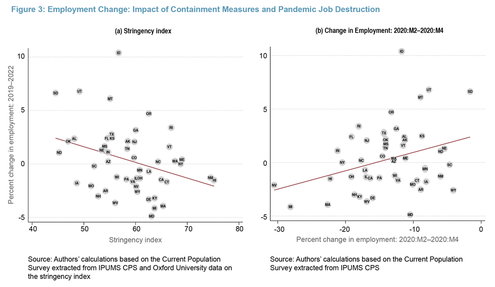
Initial univariate results are presented in Figure 3. States with more stringent measures observed slower job growth between 2019 and 2022 (3a), a situation which highlights that stringent measures may have contributed to a slower labor market recovery. Similarly, areas with a smaller decline in employment between 2020:M2 and 2020:M4 saw greater growth in employment between 2019 and 2022 (3b). However, these two mechanisms may be significantly correlated. To jointly evaluate their impact and to control for other potential contributing factors, we present results for a multiple regression model in Table 1, column 1.

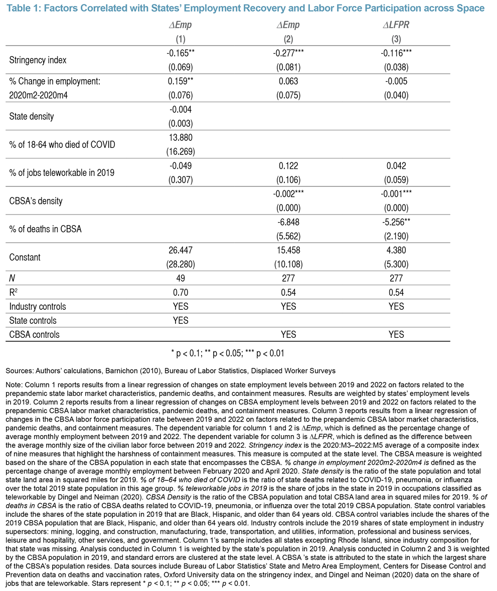
Column 1 corroborates the correlation among the stringency index, the percentage change in employment during 2020:M2–2020:M4, and the recovery of employment at the state level. An increase of one standard deviation in the stringency index (an increase of 5.65 in a 0 to 100 scale) is associated with a 1.15 percentage point decline in the percentage change in employment. Similarly, an increase of one standard deviation in the change in employment during 2020:M2–2020:M4 (representing a smaller decline) is associated with a 0.85 percentage point gain in employment between 2019 and 2022. The changes in employment during this period were sizable, ranging from -6.6 percent to 6.7 percent. Furthermore, some of the variables initially thought to affect the impact of the pandemic on the local economy, such as the number of teleworkable jobs, proxied by the share of 2019 jobs that would be considered teleworkable by the methodology presented by Dingel and Neiman (2020), and the harshness of the pandemic, measured by the number of working-age workers that have died from COVID-19 complications, appear uncorrelated to the overall recovery once other factors are taken into account.⁵ Finally, the share of the population fully vaccinated by May 2022 seems negatively correlated to economic recovery. However, we should keep in mind that the stringency index and the share of population vaccinated are highly positively correlated.

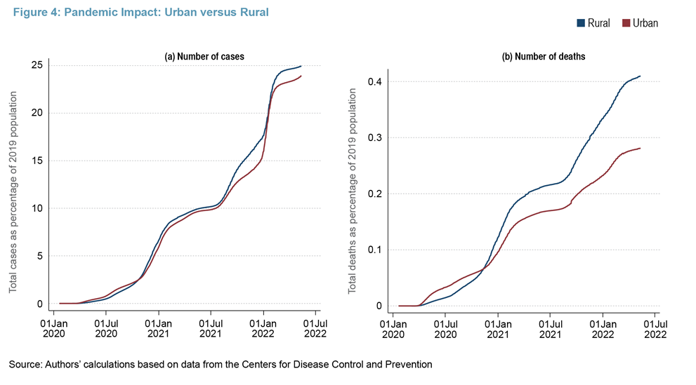
State boundaries are, however, too coarse partitions for analysis at the local-economy level. In particular, the impact of the pandemic varies significantly within a state, especially between urban and rural areas (see Figure 4). For more granular evidence across urban areas, we focus on variation across core based statistical areas (CBSAs), which correspond to metropolitan and micropolitan areas. Results are presented in Table 1, column 2. Results for the stringency index are similar to the ones obtained in column 1. An increase of one standard deviation in the stringency index (an increase of 5.34 on a 0 to 100 scale) is associated with a 1.6 percentage point decline in the change in employment levels between 2019 and 2022. Unlike in the state-level analysis, denser CBSAs are associated with slower recoveries, and the share of jobs lost in 2020 has a statistically insignificant impact once we account for other factors.

Finally, we must take into account that COVID-19 and working from home triggered some internal migration (see Whitaker, 2021). To account for migration and to further examine the potential mechanisms through which COVID-19 and its mitigation measures may have impacted the labor market, we consider the change in the labor force participation rate (LFPR) in Table 1, column 3. Since LFPR’s denominator factors in the total working-age population in the CBSA, out migration from denser CBSAs affect the ratio. Unfortunately, the Census has not yet released its population estimates for 2022. Hence, we use the working-age population reading for 2021 as a proxy for 2022. Implicitly, we assume that the bulk of the out migration resulting from COVID-19 had already happened by July 2021. Results from column 3 are similar to the ones presented in column 2. An increase of one standard deviation in the stringency index (an increase of 5.12 in a 0 to 100 scale) is associated with a 0.67 percentage point decline in the change in the LFPR between 2019 and 2022. This is a meaningful decline considering that the range of changes observed in the data goes from -6.0 percent to 4.6 percent across the CBSAs in the sample. It is worthwhile to note that the share of deaths in the CBSA seem negatively correlated with changes in LFPR. This is in line with the persistence of individuals who answered that they have been prevented from looking for a job because of the pandemic, as based on the BLS’s supplemental questions. Finally, in robustness checks, we re-run the regressions presented in column 2, including the percentage change in the CBSA’s working-age population between 2019 and 2021 as a control variable. Results were qualitatively the same and indicate that the change in a CBSA's working-age population between 2019 and 2021 does not account for the observed change in employment. Similarly, we redid the analysis presented in column 3 using the percentage change in the CBSA’s working-age population between 2019 and 2021 as the dependent variable. We find that more stringent COVID-19 containment measures are associated with lower population growth, indicating some out migration. That said, accounting for population changes does not alter the patterns previously described.

Changes in Economic Activity Across Space

There has been significant discussion in how the pandemic may have changed workers’ location as a result of remote work (telework). These new work arrangements allowed workers to move far away from their jobs and firms to hire talent at the national level (see Althoff et al., 2022; Delventhal and Parkhomenko, 2022; and Ozimek, 2022). Economic activity may have changed as demand shifts across space, as remote workers demanded goods and services in different places. To evaluate these changes across space, we calculate the location quotient for different industries and occupation groups. The location quotient for industry i in CBSA j is defined as

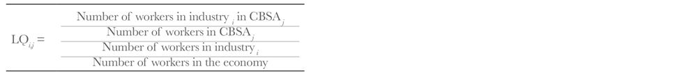
Hence, if LQ_i,j is larger than 1, it means that the CBSA is more concentrated than the economy in a particular industry. If an industry is more concentrated across space, we expect the distribution of LQs to have thicker tails, indicating larger shares of CBSAs with high and low LQs. Likewise, if an industry is evenly distributed across space, the distributions of the LQs would have thinner tails and greater density near an LQ of 1, indicating most CBSAs have similar LQs.

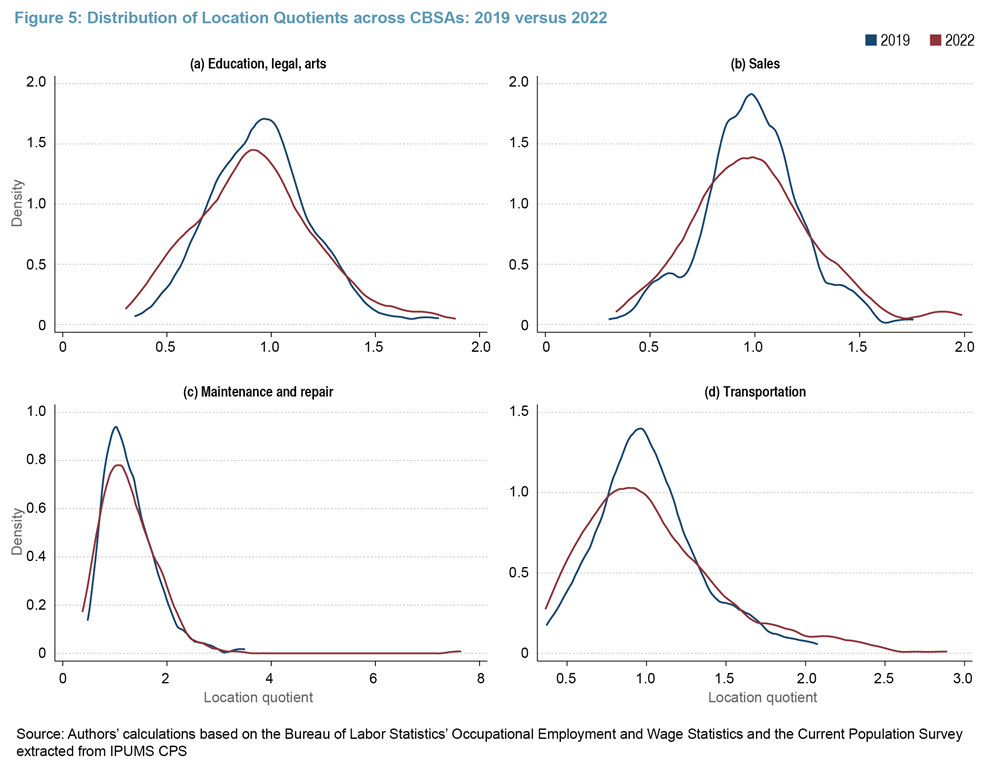
We construct LQ distributions for both industry and occupation groups for CBSAs in 2019 and 2022, and we test if they are different in statistical terms.⁶ Changes are significantly different from zero in the occupation groups of sales, maintenance and repair, transportation, and education, legal, and arts. Results are presented in Figure 5. Similarly, we see a difference that is statistically different from zero for the information industry group. In all the cases with a difference that is statistically different from zero, the later LQ distribution has thicker tails, indicating that these occupations are becoming more spatially concentrated. This concentration is at odds with the narrative that telework is making economic activity more evenly spread across space, at least in terms of the distribution of activity across urban areas. However, it is in line with an uneven labor market recovery across space, as discussed previously.

Conclusion

In this Commentary, we show that the labor market recovery from the COVID-19 recession has been uneven across space and occupations. In particular, denser metropolitan areas and those that imposed stricter measures to contain the spread of COVID-19, according to Oxford’s stringency index, have seen slower recovery on employment levels and labor force participation. While there were some changes in the distribution of economic activity across space, these changes are more in line with an uneven recovery than with a change in the productive process resulting from changes in work arrangements.

References

- Althoff, Lukas, Fabian Eckert, Sharat Ganapati, and Conor Walsh. 2022. “The Geography of Remote Work.” Regional Science and Urban Economics 93 (March): 103770. https://doi.org/10.1016/j.regsciurbeco.2022.103770.
- Dauer, Carl C. 1957. “The Pandemic of Influenza in 1918–1919.” Washington, DC: Public Health Service, National Office of Vital Statistics.
- Delventhal, Matthew J., and Andrii Parkhomenko. 2022. “Spatial Implications of Telecommuting.” https://doi.org/10.2139/ssrn.3746555.
- Dingel, Jonathan I., and Brent Neiman. 2020. “How Many Jobs Can Be Done at Home?” Journal of Public Economics 189 (S1): 104235. https://doi.org/10.1016/j.jpubeco.2020.104235.
- Forsythe, Eliza, Lisa B. Kahn, Fabian Lange, and David Wiczer. 2022. “Where Have All the Workers Gone? Recalls, Retirements, and Reallocation in the COVID Recovery.” Labour Economics 78 (S1): 102251. https://doi.org/10.1016/j.labeco.2022.102251.
- Goldman, Matt, and David M. Kaplan. 2018. “Comparing Distributions by Multiple Testing across Quantiles or CDF Values.” Journal of Econometrics 206 (1): 143–66. https://doi.org/10.1016/j.jeconom.2018.04.003.
- Hale, Thomas, Noam Angrist, Rafael Goldszmidt, Beatriz Kira, Anna Petherick, Toby Phillips, Samuel Webster, et al. 2021. “A Global Panel Database of Pandemic Policies (Oxford COVID-19 Government Response Tracker).” Nature Human Behaviour 5 (4): 529–38. https://doi.org/10.1038/s41562-021-01079-8.
- Kouchekinia, Noah, Marianna Kudlyak, Mitchell Ochse, and Erin Wolcott. 2020. “Temporary Layoffs and Unemployment in the Pandemic.” FRBSF Economic Letter 2020 (34): 01–05. https://fedinprint.org/item/fedfel/89050.
- Ozimek, Adam. 2022. “How Remote Work Is Shifting Population Growth across the US.” Economic Innovation Group. https://eig.org/how-remote-work-is-shifting-population-growth-across-the-u-s/.
- Whitaker, Stephan D. 2021. “Did the COVID-19 Pandemic Cause an Urban Exodus?” Cleveland Fed District Data Brief. Federal Reserve Bank of Cleveland. https://doi.org/10.26509/frbc-ddb-20210205.
Suggested Citation
DeLuca, Martin, and Roberto B. Pinheiro. 2023. “US Labor Market after COVID-19: An Interim Report.” Federal Reserve Bank of Cleveland, Economic Commentary 2023-04. https://doi.org/10.26509/frbc-ec-202304
This work by Federal Reserve Bank of Cleveland is licensed under Creative Commons Attribution-NonCommercial 4.0 International