

- Share
Two Approaches to Predicting the Path of the COVID-19 Pandemic: Is One Better?
We compare two types of models used to predict the spread of the coronavirus, both of which have been used by government officials and agencies. We describe the nature of the difference between the two approaches and their advantages and limitations. We compare examples of each type of model—the University of Washington IHME or “Murray” model, which follows a curve-fitting approach, and the Ohio State University model, which follows a structural approach.


The views authors express in Economic Commentary are theirs and not necessarily those of the Federal Reserve Bank of Cleveland or the Board of Governors of the Federal Reserve System. The series editor is Tasia Hane. This paper and its data are subject to revision; please visit clevelandfed.org for updates.
There are two basic types of models used by epidemiologists to forecast the path of the COVID-19 pandemic: curve-fitting and structural. Fundamentally, the difference between the two is that curve-fitting relies on patterns in the data without any inference on or assumption about the underlying mechanisms that could shape the data, while the structural approach provides a theoretical framework to guide how the data and forecasts ought to behave in other circumstances, such as with out-of-sample data or alternative policies. Both approaches have advantages and disadvantages, and—depending on the context—different approaches suit different questions a forecaster might ask.
The distinction between the two approaches is a central idea of forecasting across disciplines, and it applies not only in epidemiology, but also in economics. This Commentary illustrates the tradeoffs between the structural approach and curve-fitting via an exploration of two prominent forecasts. The first, the University of Washington’s Institute for Health Metrics and Evaluation (IHME) forecast (or the “Murray forecast,” named after its lead researcher) was used in the early stages of the US epidemic by the Centers for Disease Control and Prevention (CDC) and the White House.1 It is an example of pure curve-fitting with no underlying theory and is at one extreme of the distinction we are exploring.2 The second, the Ohio State University model, is an example of a forecast with more structure, and it uses a network approach in its underlying theoretical mechanism.3 This model has been used to guide the policy of the governor of Ohio.4
It is important to note that we are in no way conducting a “horse race” to decide which approach is best. We highlight the advantages each offers from an economist’s point of view, arguing that both approaches have their uses and help us better understand the pandemic. Further, most US COVID-19 forecasts have relied on a hybrid approach that combines elements of both types of model.
Curve-Fitting and Structural Models
Curve-fitting describes an approach in which the forecaster primarily seeks to match the available data to a function, the “curve” that gives this approach its name. This curve is then used to make predictions. No part of this approach seeks to reflect the mechanisms that generated the data; in the case of virus transmission, for example, curve-fitting tracks just the number of infections or deaths that have been observed so far.
Fitting a curve to an epidemic can be especially useful in getting an immediate estimate of the seriousness of the virus. It tends to do well when the question we wish to answer concerns how many new infections are likely in the upcoming weeks. Further, because curve-fitting does not allow for assumptions about why the data are what they are, there is no risk of obtaining predictions that are distorted by incorrect assumptions, such as assuming people will socially distance in the absence of a government mandate, for example. This problem does affect the structural approach we discuss below.
However, the cost of this simplicity is that curve-fitting is not able to employ a counterfactual scenario. In other words, there is no way to create an alternative forecast under different scenarios, an ability which is key to informed policy decision-making. Finally, curve-fitting directly fits data on deaths or infections as they unfold over time. One limitation, however, is that while other data may be available concerning related elements such as how likely the virus is to spread when an infected person wears a mask, it is not always clear with curve-fitting how to use this information, whereas a well-established structural mechanism will often guide the use of other data.
Because there are subtle and technical distinctions among definitions of “structural” in use by economists, we offer a definition here for clarity. For the purpose of this Commentary, we consider a forecast “structural” if it depends on an explicit epidemiological model in the sense that, when parameters are estimated, they admit interpretations in terms of that model. In the case of COVID-19, this can be a known or estimated mechanism by which the disease spreads from person to person or a model of the connections among people that facilitate virus transmission. In contrast with curve-fitting, a structural model emphasizes the mechanisms underlying the data. Structural models are thus based on a chosen theory of how a disease is transmitted.
While curve-fitting is useful in predicting how many new infections are likely in the near future, a structural model, on the other hand, may be able to predict the outcome of particular policies such as mandating the use of facemasks in public places or answer questions such as whether travel restrictions or bar closings are effective ways to curb the spread of the virus. Yet, to its disadvantage, using a structural approach adds complications that may limit the effectiveness of the model itself. One must define a convincing and realistic mechanism or lose accuracy in the forecast, and often such realistic mechanisms greatly increase the complexity in the estimation of the forecast.
University of Washington IHME (Murray) Model
The IHME or Murray model is a curve-fitting model.5 It has been at the peak of public awareness among COVID-19 forecasts, largely because of its use to generate one of the key forecasts used by the White House. In essence, the Murray model observes cumulative death levels and fits a curve to the data as accurately as possible. The choice of which mathematical function to use to fit the data is itself an important step in building a curve-fitting forecast. In the Murray model, the shape of the curve is given by the “error function,” which is a mathematical curve that depends on three parameters that are estimated from the data.6 The parameters are α, often explained as the rate at which the infection spreads; β, the inflection point, which may be thought of as the point at which the change in daily deaths from the previous days’ number of deaths is largest; and p, the maximum death rate experienced in the location of interest. The estimation is done by considering the evolution of the disease in the early stages and selecting the three parameters that best fit that part of the curve to the data. By continuing the function into the future using these parameters, the estimated error function then forecasts deaths in the near term.
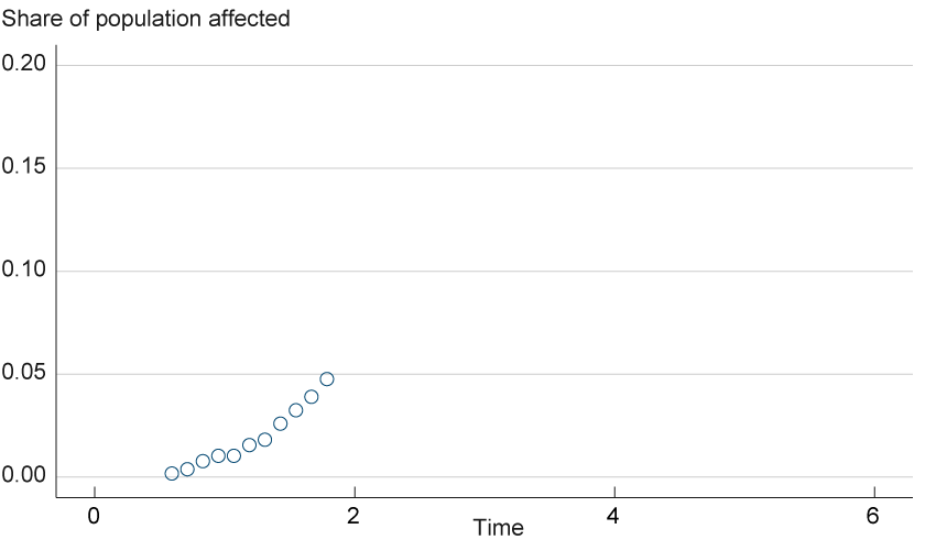
To illustrate this process, suppose we have some hypothetical data points on the proportion of deaths to infected individuals, as in figure 1. The data show a growing share of the population being affected. We can continue the path seen in the figure to generate a forecast, but it is not clear just how rapid the increase in deaths will be. This scenario illustrates just what a forecaster is faced with at the start of a pandemic. There are few data to deal with, yet the curve has to decipher as accurately as possible how the pandemic is progressing.7
Figure 1. Initial Hypothetical Data
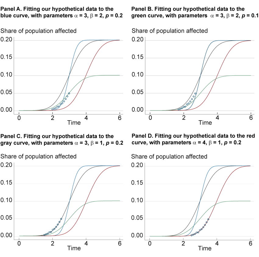
We will try to fit these data to a curve by generating a family of curves, each of which is produced by adjusting the three parameters of the error function, α, β, and p, until the combination defines a function that best fits this data. We illustrate four possible curves from this family in figure 2. We plot the same hypothetical data (which could have been measured in the early stage of an epidemic) and the same four curves in each panel, but each panel highlights one of the curves to assess how well it fits the data. Panel A shows the attempt to fit the data to the blue curve (with parameter values α = 3, β = 2, p = 0.2), while panels B, C, and D do the same for the green, black, and red curves, respectively. When we fit the data to the blue curve in panel A, the curve does not match the data very well because the infection rate of this curve accelerates faster than the data show. Nor do the data fit the curve when we decrease p to 0.1 (the green curve of panel B.) However, panels C and D show that the data fit the black and red lines, respectively, both of which look to be more accurate fits than the prior two. However, the outcomes of the panel C and D curves show very different trajectories in the path of the virus; the increase in infections is more gradual in the black line (panel C) than in the red line (panel D), which includes a higher α of 4, a difference that could imply a larger impact on the healthcare system. Further data will clarify whether the red or black curve fits better, as additional data usually aid in curve-fitting accuracy. However, the differences in the two curves illustrate the consequences of choosing the right or wrong curve.
Figure 2. Four Attempts at Fitting a Hypothetical Error Function
As with any forecast, the quality of its out-of-sample performance (i.e., using our model to fit data we have not used to build the forecast) will depend on the assumptions that have been made, some of which may prove to be accurate and others of which may not. For instance, the error function presumes that the disease will progress symmetrically, with the growth rate tailing off at the same rate at which it expanded in the early stages. If this assumption is wrong, then the forecast will be off, especially at the longer horizons. Further, compared to other curves, the error function has a strong inflection point at which the rate of infection peaks, before which it grows very quickly and after which it tails off very quickly. With the curve-fitting approach we cannot test the assumptions made by the error function family of curves until the epidemic reaches that point in its cycle. For example, we cannot test the symmetry of the error function until we have data on the epidemic where the growth rate tails off.
Figure 3 shows how the curve in March performed poorly at the longer horizons, possibly for these reasons.8 In terms of forecast performance, the main problems seem to be concerned with the error function’s longer-run performance. Note how the later projections from May and June match the data quite well into mid-July. It is only the earlier forecasts that are mistaken. This observation is consistent with our earlier point that as more data become available, the parameters are estimated more precisely.
Figure 3. Murray Model Projected US Daily Deaths
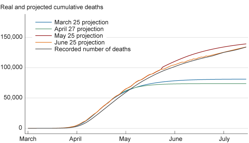
Sources: Data for projections are from the Institute for Health Metrics and Evaluation, University of Washington (www.healthdata.org/covid/data-downloads); data for recorded number of deaths are from Johns Hopkins Coronavirus Resource Center.
The parameters α, β, and p cannot be interpreted in an epidemiological framework. This is because curve-fitting does not rely on and therefore has no basis in structure. We cannot infer from an estimate of these parameters, for example, that individual contacts are decreasing. If one wants to know what would happen if a limited-contact policy such as mandatory masking, closing bars, or social distancing were adopted, the Murray forecast parameters would have only a limited ability to answer this question. This is especially true if the policy under consideration has not yet been enacted somewhere in the data set from which the forecast parameters are estimated. Rather, the three parameters in the Murray forecast embody a statistical relationship and may be estimated regardless of any context in which the curve is forecasting.
However, the parameters themselves can be enriched by being made functions of other observed variables such as geographical characteristics, policy variables, and so forth. The Murray forecast can be made very complicated as a result of these new observed variables, wherein the tradeoff that the modeler makes is one of fitting the spread of the disease more precisely (by adding more observable variables and more complex functions of these variables) versus over-fitting, where the curve fits the available data so closely that it is useless for out-of-sample predictions. Curve-fitting focuses attention on a simple tradeoff between complexity and overfitting without the distraction of whether any underlying structural model matches reality.
Structure: The Ohio State University Model
The Ohio State University model, developed at the university’s Infectious Diseases Institute, is a structural forecast that uses a network of interactions among people to model how the virus spreads.9 This network consists of people, termed “nodes.” If a node interacts with another node, that action is termed a “link” between the two nodes. Here, the model assumes a distribution about the links, and the epidemic is modeled by observing how the virus spreads from an infected person to a susceptible person based on this distribution. The model is able to use aggregate data, such as the absence of travel, average mask use, or varying degrees of human distancing that have been present over the past several months, to allow these policies to influence human behavior and subsequently to predict how that behavior will affect the distribution of links.
In contrast to the Murray curve-fitting approach, the network design of the Ohio State University model uses a theoretical epidemiological framework in the form of the SIR mechanism,10 the most commonly used model in epidemiology. The SIR, short for the Susceptible, Infectious, Removed model, assigns each individual in a population to one of the three categories (labeled S, I, or R). Its parameters may be interpreted in such a way that they can be enriched or tested with clinical data, unlike parameters in the Murray model. The model is summarized best in terms of changes to the size of each category, expressed as its respective derivative:
dS/dt = −τ × S
dI/dt = τ × S − γ × I
dR/dt = γ × I
where τ governs the infection rate and γ governs the recovery rate of individuals and S, I, and R are the number of people that are susceptible, infected, or removed, respectively. These equations are described in terms of the instantaneous rate of change so that the notation is in terms of derivatives.
The first equation describes the rate of change of the number of susceptible individuals, which is defined to be the fraction of those already susceptible who become infected, a process which happens at a rate, τ. For example, if the probability of being infected in a day, given that one is susceptible, is 1 percent, then the number of susceptible people decline in that day by 1 percent times the number of susceptible individuals in the population. Likewise, the change in the number of those infected is defined as susceptible individuals who become infected minus those currently infected who are thus removed (either because they recover and are immune or they die), a process which happens at rate γ. Lastly, the change in the number of removed individuals is the number of infected individuals who then are removed from the model. After initial values of S, I, and R are estimated, along with the rates τ and γ, this system of equations is solved for values of the numbers of S, I, and R as the system evolves over time.
This structure can use the same data on infections and deaths as the Murray approach uses, and it can incorporate additional data that might be available from medical researchers or hospitals, such as the probability of recovery and time to recovery. Further, the epidemiological model allows one to make predictive forecasts based on logical inference that the model implies. For example, one implication of the SIR model is that eventually the disease will die out because it runs out of susceptible individuals to infect with high enough probability to sustain itself (because of herd immunity often mentioned in the press). Another implication is that if a policy manages to drive the infection rate, τ, low enough, then the disease will die out before it infects the entire population. One might miss this point if only matching available data with a curve. The logical implications of the SIR model deliver policy goals in terms of the model’s parameters. For example, a vaccine should work in terms of reducing τ, and this reduction will have strong implications for the progression of the disease. This is the reason that the SIR model, or one of its variants, is so popular among epidemiologists.
The Ohio State University model extends the standard SIR model by adding a degree of useful realism. Rather than looking at the entire population and assuming everyone can possibly come into contact with anyone else in the population (the implicit assumption behind the SIR model), the Ohio State University model hypothesizes that, typically, individuals routinely have set circles of people with whom they are likely to come in contact and expresses these links within a network. For instance, one meets with the same family members or coworkers, and one is much more likely to interact at the local supermarket with someone from one’s community rather than, for example, someone from across the state. Building such ideas into a model makes the model more realistic. This extension means that an infection can take off in clusters that fill up quickly and then die out within the cluster, and other susceptible clusters then start to become infected. This result changes the dynamics of the virus’s progression, leading to very different contagion predictions than those of a standard SIR forecasting model without clusters.
The mathematics involved in modeling a network with a large population can get very complicated, and research in this area is still in its adolescence. Although much progress has been made in the last decade, there is much that is unknown about what types of contact networks are realistic with different viruses. What we do know is that ignoring networks altogether can lead to dynamics that are often not supported by the data. Further, a simple SIR model with simple network assumptions, such as assuming each person can meet anyone else in the population, can lead to misleading results, as well. In contrast, the Ohio State University model employs a concept of network analysis that has been tested and has accurately predicted the dynamics of outbreaks in previous pandemics.11 However, as shown in figure 4, the long-horizon forecasts in March proved no better than the Murray forecast.
Figure 4. Ohio State University Ohio Model Projections
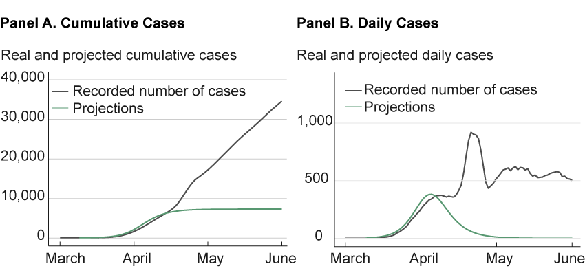
Sources: Data for projections are from a GitHub repository that provides a Python implementation of the dynamical survival analysis method used by the Ohio State University model. https://github.com/wasiur/dynamic_survival_analysis. Data for recorded number of cases are from the Johns Hopkins Coronavirus Resource Center.
The fact that both the Murray model and the Ohio State University model both missed the “second hump” of the virus points to a difference in the possible response of the two approaches to forecasting when the forecast fails at the longer horizon. The curve-fitters might go to an encyclopedia of curves and choose a set of curves that allows two humps and refit the data to the new set. The structural forecasters face a task that is more difficult, yet potentially more rewarding. They must ask the deeper question: What in our mechanism failed? They then repair the mechanism so that it allows more humps earlier in the pandemic. The potential reward is the deeper understanding of reasons for the progression of the disease, an understanding that offers possible ways to better respond effectively to the pandemic’s spread.
Importantly, structural models, such as the Ohio State University model, provide a way to allow policy to interact with the specific model. For example, in the cluster example mentioned above, people who are connected to each other tend to be connected to people who are connected to each other. Incorporating these types of connections into the model allows for topics such as contact tracing, social distancing, and business closures to be better understood and to be modeled explicitly in the forecast. A curve-fitting model, in the absence of structure, will treat all the policies in a similar fashion, adding a similar parameter for each policy without considering the insight that a structural model might deliver in which different policies affect the evolution of the disease differently.
The Structural Approach for Guiding Policy Choices
From a naïve point of view, curve-fitting might seem to offer decisive advantages in all situations. It is a straightforward and intuitive process. From this same point of view, the value of a structural approach can seem illusory. Notably, structural models of pandemics can provide misleading forecasts if the structural assumptions are wrong.12
When guiding policy, however, a structural approach is absolutely necessary because models using it provide insight into the causal relationships that predict what happens when different policies are implemented. A curve-fitting approach cannot provide causal insights. Consider a public official whose job is to decide whether to open the schools during a spike in the number of cases. On the surface, it may seem that curves could be fit as a function of policy, and then a counterfactual could be estimated by plugging in a new policy. For example, we might have data from other counties in which schools were closed or held open and use that data to estimate a forecast through a fitted curve. The official could choose “the schools are closed” curve or “the schools remain open” curve to try to predict the outcome of each policy choice. This approach presumes that there is already a rich data set with both school closures and schools held open under a robust variety of circumstances in order to extrapolate and map to our particular official’s situation. Unfortunately, this approach also confuses correlation and causality.
Modeling causality requires structure. The science of distinguishing causality from correlation is too complex to pursue here, but one result is that without a structural model, one lacks the mechanism to discuss what assumption is needed to estimate causal parameters required to make a counterfactual statement, for example, asking what would be the effect of performing a policy that is not yet in place. Without an assumption on the model, such as which school districts decide on which policies and why, measurement of correlation cannot be used to make a causal statement (in this case, if our particular official decides to close this school district, whether or not doing so will slow the infection by a predicted amount).
Data on regional policy differences and a rich structural model that identifies causality can give insights into which regions are likely to adopt safer practices in the absence of policy. One can also look at the effects (and costs) of a policy that affects the connections of specific people (such as aggressive contact tracing to isolate those connected to people who might be contagious). These effects can be compared to the effects of societal transformation, such as a popular reaction to news about a coronavirus outbreak (such as when people generally cut back on all of their contacts proportionally) or promoting wearing N95 masks throughout the population.
A final advantage offered by a more structural approach is that it provides more possible responses open to a researcher when the forecast fails. With curve-fitting, in some sense there are only two ways to correct a bad forecast: find another family of curves or re-estimate the current family of curves until the current data are fit by the best curve. In contrast, a structural model allows one to examine the entire model of behavior underlying the forecast. Does making a more sophisticated assumption about whether the public responds rationally produce a better forecast? How about the structure of the network: Is the assumption of the model too simple? Are asymptomatic infectious people important in driving the dynamics of the epidemic? Which network characteristics are most relevant in which situation? As each facet of the model is examined with different data and made more sophisticated when required, one may learn more about the mechanism of both the virus’s spread and the public’s response to the virus. The vast possibilities of mechanisms for the spread of the virus and our response to it allow the epidemiology profession in its entirety to examine and develop a set of models about virus spread that are accepted as being generally true, a situation which allows progress in handling the next pandemic when it arises.
It seems a paradox: Because so many things can go wrong with a complex structural model, it offers many opportunities for discovering what is right about possible models. When the next pandemic hits, researchers may be better prepared with a richer set of tools to combat the disease. This tradeoff, between simplicity and complexity, is true in all design endeavors, with the advantages of each often resulting in parallel research programs.
Future Developments in the Two Approaches
The early stages of the COVID-19 pandemic in the United States have taught much to both epidemiologists and economists. As can be seen in the figures 3 and 4, both approaches underestimated the strength of the COVID-19 pandemic in March 2020. In fact, almost all forecasts of the virus based on either formal curve-fitting or on more structural approaches at the beginning of the pandemic, whether by economists or epidemiologists, were widely inaccurate at the longer horizons. The COVID-19 pandemic in the United States confronted researchers with a particularly difficult set of circumstances: the large number of asymptomatic infected individuals, the lack of a uniform testing program at the national level, the lack of testing equipment at the local level, the number of those infected, the wide variety of policies, the wide variety of public response to both these policies and to the coronavirus itself, the sheer immensity and variety of economic responses, and the costs of the public response to the virus. Each of these problems individually presented both approaches with large challenges; together, they are almost overwhelming.
There has been progress in using both the curve-fitting and the structural approaches to forecast the COVID-19 pandemic. Curve-fitters are using some of the latest advances in machine-learning, such as the training of neural networks, to explore their potential for producing more accurate forecasts of the progression of the virus. Meanwhile, economists using structural models are also developing sophisticated structures of population response to the virus that can be adopted within empirical models to estimate policy costs and benefits in a straightforward manner. Other economists are using models of behavioral responses to estimate the effect of the fact that the virus is often spread by asymptomatic people. Optimal policy options and the public’s response to the virus are shown to be substantially affected by this characteristic of the current pandemic. Economists are using network models originally developed by epidemiologists to help estimate the costs of the pandemic. And epidemiologists are developing revolutionary new techniques as well.13 What is curious is that the same tradeoffs endemic to the forecasting of pandemics between structure and curve-fitting show up in other fields in which forecasting is used, particularly in economics. This perhaps should be unsurprising. Both fields involve similar foundational elements: Policy action must be decided quickly, and such policies involve costly tradeoffs.
Footnotes
- Coronavirus Task Team coordinator Deborah Birx repeatedly cited the Murray forecast as a source the White House was using in the early stages of the epidemic in the United States. Indeed, she first reported on the forecast, stating “Chris Murray ended up at the same numbers [as the White House models for previous epidemics]. So if you go on his website, you can see the concern we had, with the gray—growing number of potential fatalities.” https://trumpwhitehouse.archives.gov/briefings-statements/remarks-president-trump-vice-president-pence-members-coronavirus-task-force-press-briefing-14/. Return to 1
- Other forecasting models of the pandemic include Imperial College, London; Northeastern University; Massachusetts Institute of Technology; University of Texas at Austin; University of California, Los Angeles; Los Alamos National Laboratory; and Columbia University. The CDC reports on a number of these models at https://www.cdc.gov/coronavirus/2019-ncov/covid-data/forecasting-us.html. This list is, of course, indicative rather than exhaustive. Return to 2
- For a comprehensive overview of network models and epidemics, see Craig et al. (2020). Return to 3
- The Ohio Department of Health keeps a webpage with the Ohio State University model’s prediction on its website. It is available at https://coronavirus.ohio.gov/wps/portal/gov/covid-19/dashboards/other-resources/forecast-model. Return to 4
- The Murray model has undergone multiple alterations since its initial publication in March. We refer to the original model, Murray (2020). Details of model updates are available at http://www.healthdata.org/covid/updates. Return to 5
- More formally, the error function is defined as
p /2 (1 + 2 / √π ∫0α(τ−β exp(−τ2)dτ),
where p is the maximum death rate per location, α is the rate at which infection spreads, β is when the change in daily deaths is largest from the previous days’ number of deaths, t is the time since the death rate exceeded approximately 0, and τ is time.ths is largest from the previous days’ number of deaths, t is the time since the death rate exceeded approximately 0, and τ is time. Return to 6 - The data in figure 1 are generated using a base-case scenario of the error function above using parameters α = 3, β = 1, and p = 0.2 and a normal shock with mean 0 and standard deviation 0.001. Return to 7
- We use data provided from the Murray model’s website, https://www.healthdata.org/covid/data-downloads. We use data from Johns Hopkins Coronavirus Resource Center, https://coronavirus.jhu.edu/map.html as a comparison, which we transform into a seven-day rolling mean. Return to 8
- The Ohio State University model is described in OSU/IDI COVID-19 Response Modeling Team (2020). Data in figures are taken from https://github.com/wasiur/dynamic_survival_analysis. Return to 9
- This quality of the standard SIR model is more fully described in Craig et al. (2020). Return to 10
- See Keeling and Rohani (2008), Rand (1999), House and Keeling (2010), and, especially, Kiss, Miller, and Simon (2017) for a through discussion of the advantages of type of structure used in the Ohio State University model. The specific and highly original structure of the Ohio State University model is discussed in reference to past pandemics in KhudaBukhsh et al. (2019). Return to 11
- For an exposition of this phenomenon, see Craig et al. (2020). Return to 12
- For machine learning modeling, see Wang et al. (2020); for a sophisticated economic response in a real business cycle model, see Farboodi, Jarosch, and Shimer (2020); for the optimal policy response, see Krueger, Uhlig, and Xie (2020); for a comprehensive overview of networks and epidemiological modeling, see Kiss, Miller, and Simon (2017). Return to 13
References
- Craig, Ben, Thomas Phelan, Jan-Peter Siedlarek, and Jared Steinberg. 2020. “Improving Epidemic Modeling with Networks.” Federal Reserve Bank of Cleveland, Economic Commentary, 2020-23. https://doi.org/10.26509/frbc-ec-202023.
- Farboodi, Maryam, Gregor Jarosch, and Robert Shimer. 2020. “Internal and External Effects of Social Distancing in a Pandemic.” University of Chicago, Becker Friedman Institute for Economics, Working Paper No. 2020-47. https://doi.org/10.2139/ssrn.3580490.
- House, Thomas, and Matt J. Keeling. 2010. “The Impact of Contact Tracing in Clustered Populations.” PLoS Computatational Biology, 6(3), e1000721. https://doi.org/10.1371/journal.pcbi.1000721.
- Keeling, Matt J., and Pejman Rohani. 2008. Modeling Infectious Diseases in Humans and Animals. Princeton University Press, Princeton. https://doi.org/10.2307/j.ctvcm4gk0.
- Kiss, István Z., Joel C. Miller, and Péter L. Simon. 2017. Mathematics of Epidemics on Networks: From Exact to Approximate Models (especially Chapters 4 and 5). Springer International Publishing. https://doi.org/10.1007/978-3-319-50806-1.
- KhudaBukhsh, Wasiur R., Boseung Choi, Eben Kenah, and Grzegorz A. Rempała. 2019. “Survival Dynamical Systems: Individual-Level Survival Analysis from Population-Level Epidemic Models.” Interface Focus, 10:20190048. https://doi.org/10.1098/rsfs.2019.0048.
- Krueger, Dirk, Harald Uhlig, and Taojun Xie. 2020. “Macroeconomic Dynamics and Reallocation in an Epidemic.” 2020. National Bureau of Economic Analysis, Working Paper No. 27047. https://doi.org/10.3386/w27047.
- Murray, Christopher, J.L. 2020. “Forecasting COVID-19 Impact on Hospital Bed-Days, ICU-Days, Ventilator-Days and Deaths by US State in the Next 4 Months.” MedRxiv. Unpublished manuscript. https://doi.org/10.1101/2020.03.27.20043752.
- OSU/IDI COVID-19 Response Modeling Team. 2020. “Predicting COVID-19 Cases and Subsequent Hospital Burden in Ohio.” Ohio State University, White Paper. https://idi.osu.edu/assets/pdfs/covid_response_white_paper.pdf.
- Rand, D.A. 1999. “Correlation Equations and Pair Approximations for Spatial Ecologies.” In Advanced Ecological Theory: Principles and Applications, pp. 100–142. Blackwell Science, Oxford. https://doi.org/10.1002/9781444311501.
- Wang, Peipei, Xinqi Zheng, Jiayang Li, and Bangren Zhu. 2020. “Prediction of Epidemic Trends in COVID-19 with Logistic Model and Machine Learning Technics.” Chaos, Solitons, and Fractals, 139. https://doi.org/10.1016/j.chaos.2020.110058.
Suggested Citation
Craig, Ben R., Tom Phelan, Jan-Peter Siedlarek, and Jared Steinberg. 2021. “Two Approaches to Predicting the Path of the COVID-19 Pandemic: Is One Better?” Federal Reserve Bank of Cleveland, Economic Commentary 2021-10. https://doi.org/10.26509/frbc-ec-202110
This work by Federal Reserve Bank of Cleveland is licensed under Creative Commons Attribution-NonCommercial 4.0 International

