

- Share
How Aggregation Matters for Measured Wage Growth
Wage growth is often measured by the change in average hourly earnings (AHE), a gauge of overall wages that aggregates information on earnings and hours worked across individuals. A close look at this aggregation method demonstrates that AHE growth reflects disproportionately the profile of high-earning workers who typically display lower and less cyclically sensitive wage growth. Using data from the Current Population Survey (CPS), we adopt a different aggregation method and compute wage growth as the average of individuals’ wage growth. The analysis indicates that the CPS measure of average wage growth is significantly higher than AHE growth and that it displays a more meaningful nonlinear relationship with the Congressional Budget Office’s unemployment gap. Last, our findings do not support the claim that there was hidden slack in the labor market during the recent expansion that was restraining wage growth.

The views authors express in Economic Commentary are theirs and not necessarily those of the Federal Reserve Bank of Cleveland or the Board of Governors of the Federal Reserve System. The series editor is Tasia Hane. This paper and its data are subject to revision; please visit clevelandfed.org for updates.
Despite substantial and ongoing improvement in labor market conditions during the recent expansion, wage growth appeared to be modest relative to the degree of labor market tightening. This observation has led to concerns about workers’ ability to realize meaningful real wage growth even when labor markets are relatively strong, as well as questions about a weakened relationship between wage growth and the unemployment rate.
Measuring wage growth at the economy-wide level relies on combining or “aggregating” data across individuals. Aggregation usually involves constructing a measure of the level of overall wages, or an average wage, with wage growth computed as the change in the average wage. Among various average wage series, average hourly earnings (AHE) is a popular measure and pools information on earnings and hours worked across individuals. In this Commentary, we highlight the implications of aggregating the data in this fashion and note that AHE growth, under some simplifying assumptions, is equivalent to weighting individual workers’ wage growth by their relative earnings. Using survey data on households, we adopt an alternative aggregation scheme that equally weights individual workers’ wage growth to compute a measure of average wage growth. We then compare AHE growth to average wage growth.
We find average wage growth is consistently higher and more cyclically sensitive than AHE growth, and that the differences are largely due to the different aggregation methods. Compared to average wage growth, AHE growth over-weights high-earning workers, who tend to have lower and less cyclical wage growth.
Viewed through the lens of average wage growth rather than AHE growth, wage growth showed a notable pick-up in the aftermath of the Great Recession, and workers continue to experience significant real wage growth. Average wage growth also displays a more meaningful nonlinear relationship with labor market slack as measured by the Congressional Budget Office’s (CBO) unemployment gap. An estimated Phillips curve model yields a close alignment between recently observed and predicted values of average wage growth, a pattern that is inconsistent with claims that unmeasured labor market slack was restraining wage growth during the latter part of the recent expansion.
Growth in an Average Wage and Average Wage Growth Are Not the Same
We begin by comparing growth in an average wage—average hourly earnings (AHE)—to a measure of average wage growth that we construct, and then we highlight how differences in their construction yield different measures of wage growth and implications about the labor market. A key difference between these measures is the way each aggregates data across individuals: AHE growth aggregates data in levels to produce a measure of overall wage growth, while average wage growth aggregates data in growth rates to produce a measure of overall wage growth.
While there are several commonly used series to measure wage growth, we focus on average hourly earnings (AHE), a series produced by the Bureau of Labor Statistics (BLS) and derived from a monthly survey of business establishments. Our choice is partly based on the popularity of the series and its longstanding use in research and policy analysis. Another consideration is that AHE provides the closest analogue to our average wage growth measure and facilitates the central discussion points of the analysis.
As we will describe in more detail shortly, we examine the AHE of production and nonsupervisory workers. The AHE measure in month t is based on data collected during the relevant survey week and is computed as the ratio of total weekly earnings (Et ) to total weekly hours (Ht ):
(1) 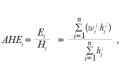
where there are n individuals, and the weekly earnings of worker i are defined as the product of the wage paid (wti) and hours worked (hti) . Equation (1) highlights that the construction of AHE uses an aggregation method that sums over the level of weekly earnings and hours worked of each individual.1 Aggregate wage growth can be measured as the percentage change in AHE.
As shown in Rich and Tracy (2019), AHE growth can be decomposed into three components involving:
(1) individual wage growth; (2) individual hours growth; and (3) a composition effect arising from individuals entering or exiting work. For ease of comparison and to identify the key difference between AHE growth and our average wage growth measure, we focus on the 12-month growth rate of AHE and consider for the moment the special case where we suppress the effects of components (2) and (3). That is, hours of work for each individual remain constant and no individual enters or exits work over the 12-month period.2 Under these strong simplifying assumptions, the 12-month growth rate of AHE (ΔAHEt+12,t ) is given by:
(2) 
where Δwit+12,t is worker i’s 12-month wage growth and (sti) is the fraction or share of earnings received by worker i relative to the total earnings of all n individuals during the survey week in month t. That is, wage growth as measured by AHE is an earnings-weighted average of individuals’ wage growth.
For our alternative measure of aggregate wage growth, we use the simple average of individuals’ wage growth. Let (wti) denote the wage paid to worker i in month t. Using the difference in log wages to measure growth, the 12-month growth rate in the wage for worker i is given by:
(3) 
Average wage growth is then calculated as:
(4) 
Both the growth in AHE and average wage growth convey information about wage gains occurring in the labor market, but a closer look at the measures reveals two important differences.
The first difference is methodological. Specifically, average wage growth equally weights each worker’s wage growth. In contrast, in the simple example we consider, the growth in AHE weights each worker’s wage growth by that worker’s earnings share. If every worker in month t has the same earnings, then the growth in AHE would equal average wage growth. However, if earnings differ across workers, then the wage growth for workers with higher earnings will receive a larger weight in the calculation of AHE growth than in the calculation of average wage growth.
The second difference concerns the particular aspects of wage growth described by the measures. From the perspective of labor market participants, average wage growth conveys information about the average wage change experienced by workers, while AHE conveys information about the change in the average wage (or, more specifically, payroll expense per hour) experienced by firms.3
Based on the methodological difference, an important consideration in comparing the two measures of wage growth is the correlation between the level of earnings and subsequent wage growth. As documented by Mincer (1974) and Becker (1975), life-cycle wage profiles are generally concave in workers’ ages. Early in their careers, workers tend to have low earnings, but high wage growth. By mid-career, workers tend to have high earnings, but lower wage growth. Finally, by late-career, workers tend to have their highest earnings, but flat to negative wage growth. Consequently, the life-cycle pattern of wages creates a negative correlation between the earnings level and wage growth of a worker. All else the same, this negative correlation will lower AHE growth below that of average wage growth.4
If the cyclical sensitivity of wages differs over the life-cycle, then the issue of aggregation will also bear upon the cyclical behavior of AHE growth and average wage growth. There is evidence that wage growth is more cyclical for young workers (Topel and Ward, 1992) and workers who have low earnings (Bils, 1985, and Blank, 1990). Both of these findings are closely related to job changing, which is more prominent among younger workers and is generally associated with large wage changes.5 Because AHE reflects disproportionately the cyclicality of wages for older, higher-earning workers, we would expect AHE growth to be less cyclical than average wage growth.
Taken together, these considerations argue that differences in aggregation methods and the associated weighting schemes for individuals’ wage growth can impact the measured change and cyclical properties of AHE growth and average wage growth. We now look to quantify these effects.
Different Behaviors
We now provide details on the AHE wage series and the micro data from the Current Population Survey (CPS) that we use to construct an average wage growth series.
The AHE series is published by the BLS using data from the Current Employment Survey—also known as the monthly establishment survey.6 This is a large stratified random sample survey of roughly 140,000 businesses and 440,000 establishments. The survey covers the private nonfarm sector. Each reporting establishment provides employment, payroll expenses, and hours for the pay period covering the twelfth day of the month for nonsupervisory workers. Payroll expenses reflect payments before deductions and include overtime, paid holidays, vacation, and sick leave. Bonuses and commissions are excluded unless they are paid monthly. As previously noted, average hourly earnings is calculated as aggregate payroll expenses divided by aggregate hours.
The CPS—also known as the household survey—is a residence-based survey where households in selected residences are interviewed for four consecutive months, rotated out for eight months, and then re-interviewed for four additional months for a total of eight interviews. Individuals can be matched across interviews so long as they do not move residences. The CPS covers around 60,000 residences. To match the coverage of the AHE series we use, we limit our calculations to workers in private, nonagricultural, nonsupervisory jobs.
Earnings information in the CPS is asked in the fourth and eighth surveys—known as the outgoing rotation samples—which are 12 months apart. Workers who are paid by the hour report their hourly wage rate. Salaried workers report their usual weekly earnings and usual weekly hours, which we use to impute their wage. For individuals who work in both periods and who do not move residences between the fourth and eighth surveys (nonmovers), we can compute their 12-month growth rates for wages and hours. For individuals who do not work in both periods or who change residences surveyed by the CPS between the fourth and eighth surveys (movers), we cannot compute their wage or hours growth. A high percentage of movers also change jobs, either voluntarily or involuntarily. Consequently, average wage growth based on the CPS will likely understate wage growth in an expansion and overstate wage growth in a recession.
We follow the convention in the earlier literature of measuring individual wage growth using the difference in log wages over the 12-month period as described in equation (3). The (CPS-based) average wage growth is the average of individual wage growth for those workers who are matched across the outgoing rotation group samples. To remove outliers, which could partly reflect measurement error, we symmetrically trim the top and bottom 1 percent of wage growth as well as hours growth estimates. Due to the smaller sample size of the CPS and to remove some volatility from the data, we report average wage growth on a 4-quarter change basis by averaging individual 12-month wage growth over the months relevant for a particular quarter.
It is worth noting that the Federal Reserve Bank of Atlanta’s Wage Growth Tracker also uses CPS wage data to construct 12-month changes, but that series differs from our average wage growth measure by reporting the median of individual wage growth. There are two reasons why we focus on the mean rather than the median. The first is that the mean offers a closer analogue to AHE growth and allows for a more direct comparison of the implied weighting schemes associated with individuals’ wage growth. The second concerns job changers. While nearly all workers change jobs once or more over their career, at any point in time job changers are a minority of workers. Consequently, the median wage growth suppresses the effects of job changing. However, as we indicated earlier, relatively large wage increases during an expansion and decreases during a recession are associated with job changing. The average wage growth, in contrast to the median, is better able to incorporate the effects of voluntary and involuntary job changing, to the extent such individuals do not move residences.
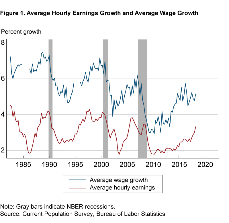
Figure 1 depicts average wage growth and AHE growth from 1983:Q1–2018:Q4.7 The gaps in the average wage growth series are due to CPS survey changes that prevent matching individuals across surveys in these years. The most prominent difference between the two wage growth measures is that average wage growth has always been higher than AHE growth over the last 35 years. For the recent period, the difference is 1.9 percentage points. The average wage growth measure indicates that in the current tight labor market workers on average are receiving sizable nominal wage gains of nearly 5 percent over the last year of the sample. This is in sharp contrast to the more modest nominal wage gains of 2¾ percent suggested by the growth in AHE.8
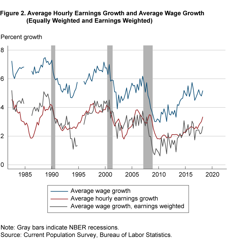
To help understand what is generating the persistent difference between the two wage growth measures, we return to the earlier discussion concerning the decomposition of AHE growth and focus on the component related to individual wage growth rates. Using the calculated individual wage growth from the workers matched across a 12-month period from the CPS data, we modify equation (4) and use the worker’s relative earnings share as the weight instead of (1/n). Figure 2 plots this earnings-weighted average-wage-growth series along with the equally weighted average-wage-growth series and the AHE-growth series. The earnings-weighted average wage growth is always lower than average wage growth. For the recent period, this difference is 2.4 percentage points. Moreover, the earnings-weighted average wage growth displays a very close correspondence with AHE growth. Consequently, the earnings weighting is extremely important in contributing to AHE growth being persistently lower than average wage growth.
Cyclical Sensitivity
While average wage growth has historically been stronger than AHE growth, there may be other differences between the series. In particular, we consider a reduced-form Phillips curve model that relates real wage growth to aggregate labor market conditions to examine the cyclical behavior of the series.9 The baseline specification is given by:
(5) 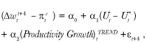
where wage growth (Δw) is measured between quarter t and quarter t + 4, inflation expectations (πe) are measured at quarter t, the unemployment gap is defined as the difference between the actual unemployment rate (U) and the CBO-estimated NAIRU (U*) measured at quarter t, trend productivity growth is measured at quarter t, and εt+4 is a mean-zero disturbance term.
We deflate both AHE growth and average wage growth using 10-year CPI inflation expectations from the Survey of Professional Forecasters and proxy trend productivity growth using a geometrically weighted average of quarterly (annualized) productivity growth rates from the business sector. To investigate possible nonlinear effects of the unemployment gap on the wage measures, we also consider specifications that differentiate between tight and slack labor market conditions, as well as increases and decreases in the unemployment gap to capture wage dynamics that may be especially important at business cycle turning points.
Figure 3 plots the resulting real wage growth for the two wage measures. One is immediately struck by the very different implications of the series for the implied real wage gains of workers. While real AHE growth indicates workers have experienced a decline in their real wage since the early 1980s, the measure of real average wage growth has been slightly above 2 percent on average over the last 35 years and suggests recent real wage gains have been particularly meaningful as labor market conditions have tightened.

The estimation results are summarized in table 1 where, prior to estimation, we make data adjustments to align the measurement of the wage measures and expected inflation series with the productivity series.10 The first three specifications focus on the growth in real AHE. From specification (1), controlling for trend productivity growth, a one percentage point decline in the unemployment gap is associated with a 35 basis point increase in real AHE growth. In specification (2), we allow for nonlinear cyclical effects depending on whether the unemployment gap is positive or negative. The results indicate only a modest (and statistically insignificant) effect of unemployment on real AHE growth in slack labor markets (a positive unemployment gap). In contrast, when labor markets are tight, a one percentage point decline in the unemployment gap is associated with a 111 basis point increase in real AHE growth.11 In specification (3), we check for “speed” effects as measured by increases or decreases in the unemployment gap over the prior quarter. The speed effects are imprecisely estimated for real AHE growth.
In specifications (4)–(6), we switch the dependent variable to our measure of real (CPS-based) average wage growth. In specification (4), we find that a one percentage point decline in the unemployment gap is associated with a 52 basis point increase in real average wage growth—a cyclical sensitivity that is nearly 50 percent higher than that of real AHE growth. In specification (5), we again allow for nonlinear effects of positive and negative unemployment gaps. Similar to the results reported for growth in AHE, the data indicate a strong nonlinearity with respect to positive and negative unemployment gaps. Now, a one percentage point decline in a positive unemployment gap is associated with a 41 basis point increase in real average wage growth, while a one percentage point decline in a negative unemployment gap is associated with a 135 basis point increase in real average wage growth. This estimate of the sensitivity of real wage growth to the unemployment rate when the unemployment gap is negative is similar in magnitude to the overall micro estimates from the earlier work of Bils (1985) and Solon Barsky, and Parker (1994).
As before, we expand the model in specification (6) to allow for speed effects measured by increases or decreases in the unemployment gap over the prior quarter. The data now document a marked difference in the speed effects associated with an unemployment gap that is rising or falling. Controlling for the level of the unemployment gap, a one percentage point increase in the unemployment gap over the prior quarter is associated with a 163 basis point slowdown in real wage growth. This result indicates that a rapidly increasing unemployment rate at the onset of a recession can exert particularly strong downward pressure on real average wage growth.12 In contrast, declines in the gap have a statistically insignificant impact on real average wage growth.
The results in table 1 also point to a sharp contrast in the features of the trend-productivity-growth coefficient and the constant term across the wage measures. The data do not reject full pass-through of trend productivity growth into real AHE growth, whereas trend productivity growth does not appear to have a statistically significant effect on real average wage growth. Instead, the regressions point to real average wage growth displaying positive, economically meaningful and statistically significant gains on average over the estimation period. Moreover, we can use information on these estimates to examine the implications for the real average wage gains of workers in a neutral labor market—that is, when the unemployment gap is equal to zero. Specifically, we calculate the total effect on wage growth associated with the constant term and the impact of trend productivity growth evaluated at its average in-sample value. On a business-sector-adjusted basis, the results indicate that real average wage growth is approximately 2½ percent in a neutral labor market, about 2 percentage points higher than the value of real AHE growth.
| (Δwtt+4 − πte) = α0 + α1(Ut − Ut*) + α2(Productivity Growth)tTREND + εt+4 | ||||||
| Variable | Real average hourly earnings (AHE) growth | Real average wage growth | ||||
|---|---|---|---|---|---|---|
| (1) | (2) | (3) | (4) | (5) | (6) | |
| (Productivity Growth)TREND | 1.118** (0.406) |
1.021** (0.390) |
1.013* (0.391) |
0.308 (0.235) |
0.218 (0.251) |
0.316 (0.201) |
| (Ut− Ut*) | −0.354** (0.114) |
−0.522** (0.081) |
||||
| (Ut − Ut*)+ | −0.255 (0.136) |
−0.206 (0.122) |
−0.411** (0.088) |
−0.328** (0.061) |
||
| (Ut− Ut*)− | −1.113** (0.388) |
−1.058** (0.401) |
−1.352** (0.320) |
−1.256** (0.294) |
||
| [(Ut − Ut*) − (Ut−1 − Ut−1*]+ | −0.774 (0.640) |
−1.628** (0.442) |
||||
| [(Ut − Ut*) − (Ut−1 − Ut−1*)]− | 1.167 (1.264) |
0.952 (0.769) |
||||
| Constant | −0.840 (0.729) |
−0.945 (0.765) |
−0.771 (0.800) |
2.173* (0.989) |
2.257* (1.062) |
2.062* (0.897) |
| Constant + α2(Productivity Growth)tTREND | 0.688** (0.221) |
2.593** (0.673) |
||||
| RMSE | 1.118 | 1.099 | 1.093 | 0.747 | 0.707 | 0.638 |
| R-square | 0.332 | 0.358 | 0.375 | 0.579 | 0.625 | 0.688 |
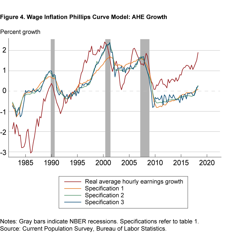
Further differences in the behavior of the wage measures and their relationships to the labor market are apparent from examining the in-sample fit of the Phillips curve models. For each series, we compare adjusted real wage growth to the predictions from the various specifications. As shown in figure 4, which focuses on (adjusted) growth in real AHE, the fitted regression lines (and the values from table 1) indicate the models are capturing little of the cyclical movements of AHE growth and that the additional predictive content from the alternative specifications is limited. Moreover, there are notable prediction errors in the earlier and later parts of the sample.
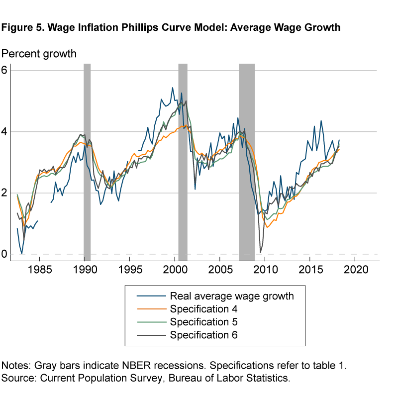
A strikingly different picture emerges from figure 5, which focuses on our measure of (adjusted) real average wage growth. Specifically, the models are better able to track the cyclical movements in real average wage growth, with the allowance for nonlinear effects of the unemployment gap especially important during episodes such as the late 1990s and the Great Recession. At present, figure 5 speaks to a remarkably close correspondence between the actual and predicted values of real average wage growth. Importantly, this finding is not consistent with the view that there was hidden slack in the labor market during the recent expansion that was restraining wage growth. Rather, a tight labor market appears to be exerting upward pressure on real average wage growth, much as it has in the past.
Conclusion
This Commentary focuses on the different aggregation methods underlying AHE growth and average wage growth and the implications for both the measured change and cyclicality of the series. We show that the behavior of average wage growth and growth in AHE can be very different, with the former measure suggesting real wages have increased at a roughly 2 percent pace since 1983. The contrast to the decline in the real wage as indicated by AHE over the same period reflects in part the overweighting in the AHE measure of older, higher-earning workers who are at the stage in their careers where they do not typically experience real wage gains.13
Another important aspect of the analysis concerns the role of the labor market in the wage growth process. Compared to growth in real AHE, real average wage growth displays a more meaningful nonlinear relationship with the unemployment gap. In particular, real average wage growth responds much more to tight labor market conditions than to slack labor market conditions, although the initial movements from the trough of an unemployment rate cycle can exert significant restraint on wage growth.
Many commentators rely on average wage measures, such as AHE, to inform them about the state of the labor market. Our analysis is not intended to be dismissive of such measures. However, it does serve as a reminder that it is important to understand the construction of wage measures and to take differences in measures into account to gauge their suitability for particular purposes.
Footnotes
- Because AHE pools data on earnings and hours worked across individuals, it provides an average wage measure whose construction does not require information on individuals’ wages to be observed separately. Return to 1
- As we discuss later, the 12-month horizon relates to the reporting of earnings information in the Current Population Survey (CPS). We relax these special assumptions for the subsequent analysis and use the as-published AHE growth rate. Return to 2
- Importantly, our statement concerning AHE should not be interpreted as a judgment about the validity or reliability of AHE as a measure of marginal cost or its specific linkage to the pricing decisions of firms. Return to 3
- Our focus on the life-cycle profile of a worker abstracts from other factors that can affect earnings and wage growth, such as inflation. Return to 4
- As noted by Jacobson, LaLonde, and Sullivan (1993), job changers tend to receive relatively large wage increases during an expansion and relatively large wage declines during a recession. The former finding is referred to as the cyclical upgrading hypothesis and is a primary source of wage growth early in a worker’s career. Cyclical upgrading can reflect a better matching of workers and firms, but the observed increase in a worker’s wage does not necessarily imply that the firm has raised its wage—the worker’s higher productivity on the new job can justify the higher wage. The relatively large wage declines during recessions among job changers primarily reflect the net effects of job displacements, as workers who lose jobs usually have lower subsequent wages. Return to 5
- See the BLS: Handbook of Methods (2018). Return to 6
- The sample period is based upon the availability of the CPS data, which we take from the Federal Reserve Bank of Atlanta’s Wage Growth Tracker website. We report AHE growth on a 4-quarter-change basis following the same procedure used for average wage growth. Return to 7
- Rich and Tracy (2019) calculate a CPS(-based) AHE to examine the reliability of using the CPS wage data for the comparative analysis. The CPS AHE uses all workers reporting a wage or salary in a month and is calculated as aggregate CPS weekly earnings divided by aggregate CPS weekly hours. They construct 12-month changes, smooth the series, and then compare growth rates of the CPS AHE and the BLS AHE starting in 1984. Apart from two positive spikes in the CPS AHE that do not exist in the BLS AHE, the CPS measure tracks the BLS AHE growth relatively closely, but with more variability due to the smaller sample sizes. We view the results as justifying our use of the CPS wage data and reinforcing our view that differences in the behavior of the two wage measures can coexist due to their different construction and focus. Return to 8
- Hooper Mishkin, and Sufi (2019), Leduc and Wilson (2019), and Kumar and Orrenius (2016) examine state-level data to try to better identify possible nonlinearities in Phillips curve models. While our subsequent analysis documents that real average wage growth displays a higher cyclical response than real AHE growth, this difference cannot be attributed solely to aggregation effects. The cyclicality of AHE growth also depends on composition effects that reflect the wages of workers entering and exiting employment relative to the wages of continuing workers. However, Rich and Tracy (2019) use similar data and find that aggregation effects contribute slightly more than composition effects to the cyclical difference in the two wage growth measures. Return to 9
- We would expect real product wages (real wages defined relative to the price of business output) to rise over time with business-sector productivity rather than real consumption wages (real wages defined relative to consumer prices). However, our expected inflation measure is in terms of CPI inflation. As a result, the expected inflation series that we use to deflate wage growth equals the reported survey measure less the average differential between the CPI and business output inflation series since 1983 (our estimation period). In addition, neither our CPS-based wage measure nor AHE has a comparable productivity measure; accordingly, the productivity trend in the average-wage-growth and AHE equations is assumed to equal business-sector trend productivity adjusted for the average differential between each of these series and growth in compensation per hour in the business sector. Return to 10
- Hooper, Mishkin, and Sufi (2019) find evidence of nonlinear effects of positive and negative unemployment gaps on the growth of AHE over the period 1954–2018. However, they find the nonlinearity disappears over the period 1994–2018. An implication of this nonlinearity is that the reported variation in the literature of the estimated cyclical effect (estimated assuming a linear effect) may reflect the choice of the sample period and the relative number of positive and negative unemployment gaps in the data. Return to 11
- While speed effects are generally small in magnitude, they were an important factor starting around the time of the Great Recession. The speed effects turned positive in 2007:Q3 and reached a maximum value of 1.4 percentage points in 2009:Q1, which, based on the model estimates, restrained average wage growth by over 2¼ percentage points over the next four quarters. The speed effects remained positive until 2010:Q1. Using a price inflation Phillips curve model, Stock and Watson (2010) and Ashley and Verbrugge (2019) find that sharp rises in the unemployment rate are also associated with weak inflation. Return to 12
- As a reminder, these statements reflect the behavior of the series in the absence of any business-sector adjustment procedures. Return to 13
References
- Ashley, Richard, and Randal Verbrugge. 2019. “Variation in the Phillips Curve Relation across Three Phases of the Business Cycle.” Federal Reserve Bank of Cleveland, Working Paper No. 2019-09. https://doi.org/10.26509/frbc-wp-201909.
- Becker, Gary S. 1975. Human Capital. New York, Cambridge University Press.
- Bils, Mark J. 1985. “Real Wages over the Business Cycle: Evidence from Panel Data.” Journal of Political Economy, 93(4): 666-689. https://doi.org/10.1086/261325.
- Blank, Rebecca M. 1990. “Why Are Wages Cyclical in the 1970s?” Journal of Labor Economics, 8(1): 16-47. https://www.jstor.org/stable/2535297.
- Bureau of Labor Statistics. 2018. “Chapter 2. Employment, Hours, and Earnings from the Establishment Survey.” In BLS Handbook of Methods. Washington DC.
- Hooper, Peter, Frederic S. Mishkin, and Amir Sufi. 2019. “Prospects for Inflation in a High Pressure Economy: Is the Phillips Curve Dead or Is It Just Hibernating?” US Monetary Policy Forum. The University of Chicago Booth School of Business, Initiative on Global Markets. https://doi.org/10.3386/w25792.
- Jacobson, Louis S., Robert J. LaLonde, and Daniel G. Sullivan. 1993. “Earnings Losses of Displaced Workers.” American Economic Review, 83 (September): 685-709.
- Kumar, Anil, and Pia M. Orrenius. 2016. “A Closer Look at the Phillips Curve Using State-Level Data.” Journal of Macroeconomics, 47, Part A: 84-102. https://doi.org/10.1016/j.jmacro.2015.08.003.
- Leduc, Sylvain, and Daniel J. Wilson. 2019. “Does Ultra-low Unemployment Spur Rapid Wage Growth?” Federal Reserve Bank of San Francisco, Economic Letter, 209-02.
- Mincer, Jacob. 1974. Schooling, Learning, and Earnings. National Bureau of Economic Research.
- Newey, Whitney, and Kenneth West. 1987. “A Simple, Positive Semi-definite, Heteroskedasticity and Autocorrelation Consistent Covariance Matrix.” Econometrica, 55(3): 703-708. https://doi.org/10.2307/1913610.
- Rich, Robert, and Joseph Tracy. 2019. “The Effects of Aggregation on Wage Growth.” Unpublished manuscript.
- Solon, Gary, Robert Barsky, and Jonathan A. Parker. 1994. “Measuring the Cyclicality of Real Wages: How Important Is Composition Bias?” Quarterly Journal of Economics, 109(1): 1-25. https://doi.org/10.2307/2118426.
- Stock, James H., and Mark W. Watson. 2010. Modeling Inflation after the Crisis.” Federal Reserve Bank of Kansas City, Proceedings—Economic Policy Symposium—Jackson Hole, 173-220.
- Topel, Robert H., and Michael P. Ward. 1992. “Job Mobility and the Careers of Young Men.” Quarterly Journal of Economics, 107(2): 439-479. https://doi.org/10.2307/2118478.
Suggested Citation
Morris, Michael, Robert W. Rich, and Joseph Tracy. 2020. “How Aggregation Matters for Measured Wage Growth.” Federal Reserve Bank of Cleveland, Economic Commentary 2020-19. https://doi.org/10.26509/frbc-ec-202019
This work by Federal Reserve Bank of Cleveland is licensed under Creative Commons Attribution-NonCommercial 4.0 International

