Cyclical versus Acyclical Inflation: A Deeper Dive

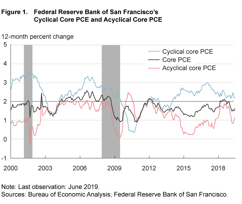
Inflation rates incorporate price changes for a wide variety of goods and services that can behave in different ways. Recent research has highlighted that the inflation rates for some categories of goods and services are relatively responsive to economic conditions, implying that they are “cyclically sensitive,” while inflation rates for other categories tend not to vary with the state of the economy and are relatively “acyclical.” Looking at the major components that comprise inflation in the price index for personal consumption expenditures excluding food and energy (core PCE inflation), the Federal Reserve Bank of San Francisco publishes a cyclical core PCE inflation series that trended up from its low point in 2010 until the beginning of 2017; see figure 1. But since that time, this cyclical core PCE inflation series has decelerated noticeably and has stabilized well below its pace from earlier in the expansion, in spite of ongoing strong payroll growth and declines in the unemployment rate, raising questions about the stability of the Phillips curve or the extent to which slack has been taken up in the economy.

In this Commentary, I show that this apparent recent tension between the perceived strength of the labor market and cyclical core PCE inflation can be resolved by conducting the analysis at a finer level of disaggregation. Instead of using 14 major components of core PCE inflation, I determine the cyclical sensitivity of 154 disaggregated subcomponents within those 14 major components and derive alternative measures of cyclical and acyclical core PCE inflation. This deeper dive allows for a more precise assessment of cyclicality because it does not assume that all subcomponents within a given component share the same cyclicality. The resulting cyclical core PCE inflation series shows that recent price pressures remain on a firming trend, commensurate with a strengthening labor market. Furthermore, the cyclical category’s contribution to core PCE inflation currently matches this category’s contribution over the period 2002–2007, a time when core PCE inflation averaged 2 percent on a sustained basis. By contrast, the inflation rate in the newly constructed acyclical category remains subdued and is a key factor weighing on core PCE inflation. In the context of a simple forecasting exercise, I show that a modest firming in acyclical core PCE inflation to a level more in line with its average over the past eight years, combined with ongoing strength in the labor market, would be enough to return core PCE inflation to 2 percent within approximately one year.

Linking Inflation and Slack at the Component Level

At the aggregate level, the empirical relationship between inflation and economic activity appears to have considerably weakened over time, suggesting that a changing set of predictors helps to explain inflation dynamics over different time periods (see, for example, Koop and Korobilis, 2012). This weakening in the Phillips curve relationship at the aggregate level has led researchers (see, for example, Stock and Watson, 2019) to examine whether there is a more stable relationship at the component, sectoral, or disaggregate level.

The idea of examining the sensitivity of prices to economic slack at a relatively disaggregated level is an old one; some examples include Hubrich (2005), Bryan and Meyer (2010), and Peach et al. (2013).¹ However, the idea has recently received renewed interest as inflation has remained subdued even though the unemployment rate has fallen to a nearly 50-year low and is below most estimates of its natural rate. Mahedy and Shapiro (2017) and Shapiro (2018) examine 14 high-level components of core PCE inflation and divide those components into cyclical and acyclical inflation categories by looking at the strength of each component’s relationship to economic activity.² Stock and Watson (2019) examine PCE inflation and construct a cyclically sensitive inflation series using 17 high-level components.³ Struyven (2017) goes down one level of disaggregation, looking at 50 subcomponents of core PCE inflation to distinguish between the cyclical and acyclical (more precisely, less cyclical) categories.⁴

Cyclical and Acyclical Inflation Using Finer Disaggregation

In this analysis, I go down one level of disaggregation further than Struyven (2017) to separate more finely the cyclal and acyclical categories of core PCE inflation. To determine whether each disaggregated subcomponent is cyclical or acyclical with respect to economic activity, I follow a strategy similar to Mahedy and Shapiro’s (2017) and estimate the relationship between the disaggregated subcomponent and labor market slack prior to the start of the Great Recession. For the purpose of the current analysis, one advantage of creating groupings based on the sample prior to the Great Recession is that it is possible to assess whether the cyclical and acyclical categories have continued to behave as expected following the Great Recession.

I use a very parsimonious Phillips curve formulation because the primary aim of my analysis is simply to identify whether each disaggregated subcomponent has a statistically significant relationship with labor market slack. To achieve that, I follow three steps.

First, for each disaggregated subcomponent denoted by j, I estimate the regression:

π_j,t = α_j + β_j x_t + e_j,t.

Inflation π_j,t is measured as the 12-month inflation rate of the subcomponent. The unemployment gap is computed as the overall unemployment rate U_t minus the Congressional Budget Office’s (CBO) estimate of the long-run unemployment rate, U_t^N.⁵ To incorporate the fact that I am using 12-month inflation rates and some components may have a delayed response to labor market slack, I use for my economic activity variable the average unemployment gap over the preceding 18 months:

The estimation period is based on data from July 1986 through December 2007.⁷ The notation indicates that the regression coefficients α_j and β_j and the regression residuals e_j,t are specific to the disaggregated subcomponent j.

Second, I examine the slope of the Phillips curve for each subcomponent. If the estimated coefficient β_j for the unemployment gap is negative and statistically significant at the 10 percent level, I classify the subcomponent as belonging to the cyclical category. Otherwise, I classify it as belonging to the acyclical category.

Third, I construct inflation rates for the cyclical and acyclical categories. The 12-month inflation rates for each category are aggregated up using the subcomponents’ 12-month inflation rates and their expenditure weights (that is, the relative share of nominal spending on the subcomponent among all subcomponents in what constitutes core PCE) to produce cyclical core PCE inflation and acyclical core PCE inflation. For the sake of comparison in highlighting the role of disaggregation in the exercise, I repeat the above three steps but this time I use the 14 higher-level components of core PCE inflation. I denote the resulting cyclical and acyclical inflation rates as “cyclical core (higher-level)” and “acyclical core (higher-level),” respectively.⁸

As of June 2019, the share of core PCE components belonging to the cyclical category using the finer level of disaggregation was roughly 40 percent. This cyclical share is slightly higher than the share that would be calculated using only the 14 higher-level components, but the underlying composition is different. For example, the classification based on 14 higher-level components flags the entire healthcare services sector as belonging to the acyclical category. That is, all the subcomponents of the healthcare services sector are implicitly assumed to be acyclical. By contrast, the classification based on the detailed 154 subcomponents flags the nursing home subcomponent of the healthcare services sector as cyclical even though all other subcomponents of healthcare services are categorized as belonging to the acyclical category. In the case of healthcare services inflation, the differences across the two approaches are small, but differences can be more significant in other components. A bigger difference is for the recreational goods and vehicles sector, wherein roughly half of the subcomponents are flagged as cyclical based on the detailed subcomponent-level examination, while the entire component is classified as acyclical based on the higher-level components.

Figure 2 plots the cyclical and acyclical core PCE inflation series constructed using the more disaggregated (finer-level) subcomponents along with those constructed at a higher level of aggregation. Both of the cyclical series share common features, as do both of the acyclical series, but they are also subject to some differences. Notably, both cyclical core inflation series firmed in line with improving labor market conditions from 2010 through the beginning of 2017. However, since the start of 2017, only the cyclical core inflation series based on the finer level of disaggregation has continued on a firming trend, and it registered 2.9 percent as of June 2019, while the cyclical measure based on the higher (less granular) level of aggregation has actually shown some deceleration, and most recently it registered 2.2 percent.

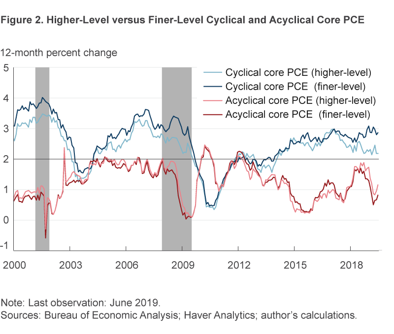
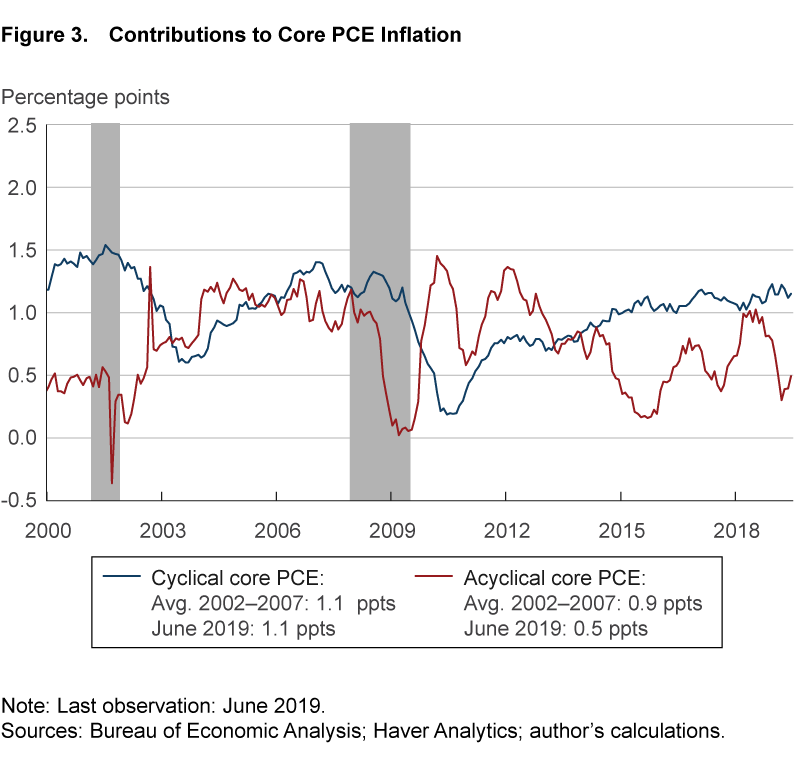
Figure 3 plots the contributions of the cyclical and the acyclical categories to core PCE inflation. As of June 2019, cyclical core inflation categories contributed 1.1 percentage points and acyclical core inflation categories contributed 0.5 percentage points. The contribution from the cyclical categories is identical to the average contribution of 1.1 percentage points over the period 2002–2007, a period during which core PCE inflation averaged 2 percent on a sustained basis. By contrast, the contribution to core PCE inflation from the acyclical categories remains quite subdued, well below its average contribution of 0.9 percentage points over the period 2002–2007, a situation which is contributing to weak core PCE inflation.

Key Drivers of Acyclical and Cyclical Inflation

Among the acyclical categories, the markedly low inflation rate is primarily driven by very low inflation rates in the subcomponents of the healthcare services sector. The disaggregated components underlying the healthcare sector that are identified as belonging to the acyclical category collectively receive the largest weight (roughly 29 percent) in the construction of the acyclical index. Shapiro (2018), Mahedy and Shapiro (2017), and Dolmas (2016) note the role of government legislation as the primary contributor to the persistently low inflation rates in the healthcare services sector. Mahedy and Shapiro (2017) and Dolmas (2016) cite reasons to believe that subdued inflation in the healthcare services category is likely to continue going forward, which would weigh on acyclical core inflation (and thus overall core inflation).

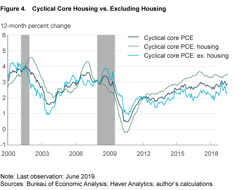
By contrast, housing is a key driver of cyclical inflation. Five of the seven disaggregated subcomponents underlying the housing sector are identified as being cyclically sensitive, and these five subcomponents collectively constitute 44 percent of cyclical core PCE inflation. Moreover, these housing subcomponents tend to be more cyclically sensitive than other subcomponents. Figure 4 plots inflation rates for cyclically sensitive housing components and for cyclically sensitive core components excluding housing. After falling into negative territory in 2010, inflation among the cyclically sensitive housing subcomponents rebounded strongly as the labor market recovered and has been running about 1 percentage point higher than inflation among the other cyclically sensitive subcomponents for most of the expansion.

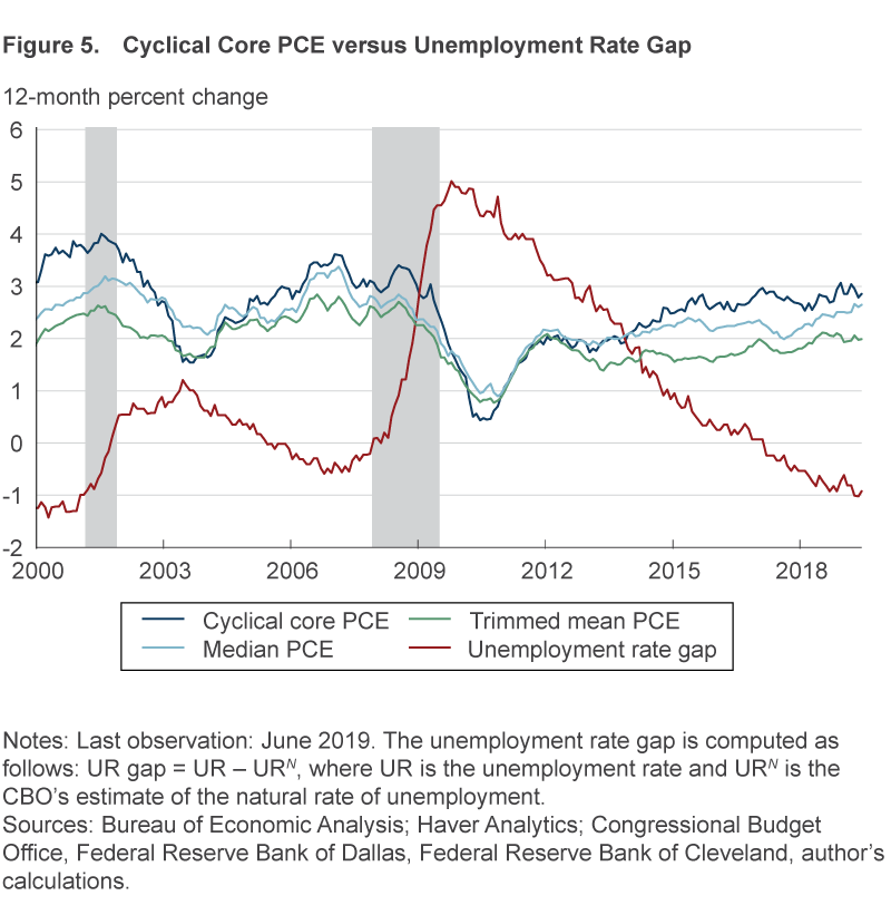
The fact that cyclically sensitive inflation rates are heavily influenced by housing categories is not unique to these specific indicators. Housing tends to be an important category when computing median inflation rates, such as the median CPI or median PCE; see, for example, Bednar and Knotek (2014) and Carroll and Verbrugge (2019). In general, inflation trend estimators such as the median CPI, trimmed-mean CPI, median PCE, and trimmed-mean PCE have a strong connection to labor market slack (for example, Ball and Mazumder, 2019; Carroll and Verbrugge, 2019). Stock and Watson (2019) suggest that this strong association with economic slack comes from the large role that the highly procyclical housing component plays in their calculation. Figure 5 plots the unemployment gap and cyclical core PCE inflation alongside median PCE inflation (based on Carroll and Verbrugge, 2019) and trimmed-mean PCE inflation. The latter three series share similar trends and are highly correlated with each other, and they are strongly negatively correlated with the unemployment gap, even though the median PCE and trimmed-mean PCE inflation rates do not use the unemployment gap to inform their construction.

Looking Ahead

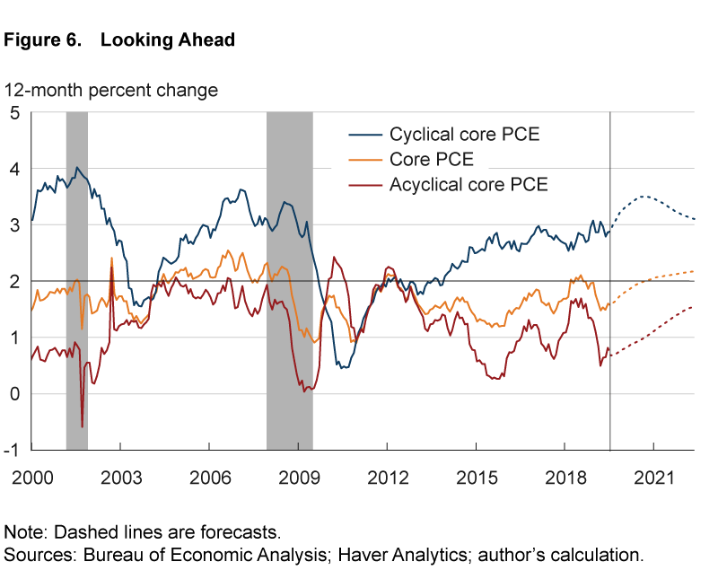
It is natural to ask what might happen going forward. Will cyclical inflation continue to firm with tightening labor markets? Is subdued acyclical inflation here to stay? To formally answer these questions, I construct a small-scale monthly vector autoregressive (VAR) model consisting of three variables: cyclical core PCE inflation, acyclical core PCE inflation, and the unemployment gap.⁹ The model consists of equations relating the current value of each variable to past values of all the variables. A statistical model of this sort formally characterizes the historical relationship among the model variables. I estimate the coefficients of the model using data from January 1985 through June 2019 and then generate forecasts for July 2019 through June 2022.¹⁰

This simple model projects that the labor market will remain quite tight through 2020. For example, the unemployment gap moves only a little, from −1.0 percentage point in June 2019 to −0.9 percentage points by June 2020. The model sees the tight labor market as exerting further upward pressure on cyclical core PCE inflation, while acyclical inflation also is projected to move up from its current low level. Figure 6 plots the forecasts of cyclical core PCE inflation, acyclical core PCE inflation, and a composite forecast of core PCE inflation using the components’ weights available as of June 2019. Cyclical core PCE inflation is projected to rise to about 3.5 percent by the middle of 2020, the point at which core PCE inflation is projected to rise to 2 percent. At that time, acyclical core PCE inflation remains quite subdued, at 0.9 percent, up only marginally from its current value and below its average of 1.1 percent over the past eight years. Thus, this forecast highlights that a modest firming in acyclical core PCE inflation combined with ongoing strength in the labor market would be enough to return core PCE inflation to 2 percent within approximately one year.

Conclusion

The analysis of this article reiterates the conclusion drawn by Williams (2019) in that the Phillips curve relationship continues to be alive and well for categories of goods and services that have historically been responsive to overall labor market conditions. While the results based on higher-level aggregates point to a recent step down in cyclically sensitive inflation, I find that a measure of cyclically sensitive inflation based on highly disaggregated data has continued on a firming trend in recent years in line with a strengthening labor market.

As also highlighted by previous researchers, most of the current weakness in core PCE inflation is concentrated in components on which the state of the labor market historically has had a limited influence on inflation rates, for example, the majority of healthcare services inflation. I show in the context of a forecasting exercise that going forward a modest firming in acyclical core PCE inflation combined with ongoing strength in the labor market would help to lift cyclical inflation further and return core PCE inflation to 2 percent within approximately one year.

References

- Babb, Nathan R., and Alan K. Detmeister, 2017. “Nonlinearities in the Phillips Curve for the United States: Evidence Using Metropolitan Data.” Finance and Economics Discussion Series, 2017-070. https://doi.org/10.17016/FEDS.2017.070
- Ball, Laurence, and Sandeep Mazumder. 2019. “The Nonpuzzling Behavior of Median CPI Inflation.” NBER Working Paper no. 25512. https://doi.org/10.3386/w25512
- Bednar, William, and Edward S. Knotek II. 2014. “What’s Up in Inflation? Shelter and OER.” Federal Reserve Bank of Cleveland, Economic Trends.
- Bryan, Michael F., and Brent Meyer. 2010. “Are Some Prices in the CPI More Forward Looking than Others? We Think So.” Federal Reserve Bank of Cleveland, Economic Commentary 2010-02. https://doi.org/10.26509/frbc-ec-201002
- Carroll, Daniel, and Randal Verbrugge. 2019. “Behavior of a New Median PCE Measure: A Tale of Tails.” Federal Reserve Bank of Cleveland, Economic Commentary, 2019-10. https://doi.org/10.26509/frbc-ec-201910
- Dolmas, Jim. 2016. “Health Care Services Depress Recent PCE Inflation Readings.” Federal Reserve Bank of Dallas, Economic Letter, 11(11).
- Fitzgerald, Terry, Brian Holtemeyer, and Juan Pablo Nicolini. 2013. “Is There a Stable Phillips Curve After All?” Federal Reserve Bank of Minneapolis, Economic Policy Paper, 13-6.
- Hubrich, Kirstin. 2005. “Forecasting Euro Area Inflation: Does Aggregating Forecasts by HICP Component Improve Forecast Accuracy?” International Journal of Forecasting, 21(1):119–136. https://doi.org/10.1016/j.ijforecast.2004.04.005
- Koop, Gary, and Dimitris Korobilis. 2012. “Forecasting Inflation Using Dynamic Model Averaging.” International Economic Review, 53(3): 867–886. https://doi.org/10.1111/j.1468-2354.2012.00704.x
- Mahedy, Tim, and Adam Shapiro. 2017. “What’s Down with Inflation?” Federal Reserve Bank of San Francisco, Economic Letter, 2017-35.
- Peach, Robert, Robert Rich, and Hendry Linder. 2013. “The Parts Are More Than the Whole: Separating Goods and Services to Predict Core Inflation.” Federal Reserve Bank of New York, Current Issues in Economic and Finance, 19(7).
- Shapiro, Adam. 2018. “Has Inflation Sustainably Reached Target?” Federal Reserve Bank of San Francisco, Economic Letter, 2018-26.
- Stock, James H., and Mark W. Watson. 2019. “Slack and Cyclically Sensitive Inflation.” NBER Working Paper no. 25987. https://doi.org/10.3386/w25987
- Stock, James H., and Mark W. Watson. 2016. “Core Inflation and Trend Inflation.” Review of Economics and Statistics, 98(4): 770–784. https://doi.org/10.1162/rest_a_00608
- Struyven, Daan. 2017. “US Daily: Which Prices Still Respond to Slack?” Goldman Sachs ER.
- Tallman, Ellis W., and Saeed Zaman. 2017. “Forecasting Inflation: Phillips Curve Effects on Services Price Measures.” International Journal of Forecasting, 33: 442–457. https://doi.org/10.1016/j.ijforecast.2016.10.004
- Williams, John C. 2019. Discussion of “Prospects for Inflation in a High Pressure Economy: Is the Phillips Curve Dead or Is It Just Hibernating?” by Peter Hooper, Frederic S. Mishkin, and Amir Sufi. Speech at the US Monetary Policy Forum, New York City. https://www.newyorkfed.org/newsevents/speeches/2019/wil190222
Suggested Citation
Zaman, Saeed. 2019. “Cyclical versus Acyclical Inflation: A Deeper Dive.” Federal Reserve Bank of Cleveland, Economic Commentary 2019-13. https://doi.org/10.26509/frbc-ec-201913
This work by Federal Reserve Bank of Cleveland is licensed under Creative Commons Attribution-NonCommercial 4.0 International