Comments on “The Equilibrium Real Funds Rate: Past, Present, and Future.”

It is a real pleasure for me to participate in this year’s Monetary Policy Forum. As an attendee of this event for the past several years, I have been very impressed with the organizers’ ability to choose a year in advance the topic that turns out to be the issue policymakers are grappling with at the time the forum rolls around. Once again, the organizers have been able to do this, with the important paper by Jim Hamilton, Ethan Harris, Jan Hatzius, and Ken West. Another example of the value of being forward looking when it comes to monetary policy!

In the time I have, I will discuss some of the highlights of the paper – some of which the authors have laid out as “lessons learned” from history. I’ll focus on measurement and implications for policy. Taking their lead, I’ll present five of my own lessons spurred by reading their interesting paper. Of course, the views I’ll present today are my own and not necessarily those of the Federal Reserve System or my colleagues on the Federal Open Market Committee.

Measurement

The authors have done a very good job of examining the question, “Is there a new neutral or equilibrium real federal funds rate?” This is a deceptively simple question that hits on bigger issues such as whether the U.S. has drifted into “secular stagnation” and what the implications for monetary policy normalization are.

The first part of the paper is a thorough analysis of what the historical data and record can tell us. The authors have amassed an impressive data set on 21 countries, with annual data in some cases going back to 1858 and quarterly data back to 1958. Where the data are available, the authors use the discount rate set by the central bank as the interest rate of interest; in some cases, they have spliced together series. For example, in the U.S. for the annual dataset they use the discount rate over 1914-1953 and the average fed funds rate during the last month of the year from 1954 to present. As anyone who has put together data sets for research knows, this effort is not trivial.

Of course before the empirical analysis can commence, it is important to understand what is meant by the “equilibrium federal funds rate” or more generally, the “equilibrium policy rate.” It is a fuzzy concept. There are several definitions in the literature. Moreover, several different terms in the literature, such as the equilibrium rate of interest, natural rate of interest, and neutral rate of interest, refer to the same object.

The paper’s definition is one that many economists use: the equilibrium real rate, r*, is that level of the policy rate that is consistent with full employment and stable inflation in the medium term. Sometimes instead of full employment a zero output gap or growth at potential is used. Presumably the stable inflation rate referred to is the policymakers’ target inflation rate. What’s undefined here is the meaning of “medium term.”

This r* is an important concept in monetary policy as it gives one a way to think about the degree of policy accommodation. For example, in a Taylor rule,

The big issue is that the equilibrium real rate, r*, is unobserved. Incidentally, so are the level of potential output and the natural rate of unemployment, which loom large in monetary policy discussions. The fact that r* is unobserved has been recognized by many economists over many decades. The authors explore several time-series approaches to estimating the real rate.

One approach is to estimate the real rate using averages over a cycle or longer of estimates of the ex ante real rate, defined as the nominal interest rate minus expected inflation,

If policymakers are setting the nominal interest rate, so that on average, the output gap (or unemployment gap) is zero, inflation is equal to target, and expected inflation is equal to target, then the ex ante real interest rate will equal the equilibrium real rate as defined by the authors. To see this, suppose policymakers are following a simple Taylor rule, then:

The authors’ empirical investigation indicates that estimates of the ex ante real rate have varied considerably over time. They show that the correlations between estimates of the ex ante real rate and output growth vary over the sample period and are sensitive to the time period examined and countries included. They also include a narrative review of the history of the U.S. ex ante real rate. This is interesting because it points out some of the factors that theory tells us might influence the real rate of interest. Based on this analysis, drawing on the connection between the ex ante real rate and the equilibrium rate, the authors conclude that it would be a mistake to estimate the equilibrium rate using long historical averages (this is their history lesson 2).

It is hard to dispute this and I don’t find it surprising. Indeed, Wicksell, in his seminal work Interest and Prices, says:

"The natural rate is not fixed or unalterable in magnitude...In general, we may say, it depends on the efficiency of production, on the available amount of fixed and liquid capital, on the supply of labour and land, in short on all the thousand and one things which determine the current economic position of a community; and with them it constantly fluctuates."

- Knut Wicksell, Interest and Prices, 1898, p. 106

Which brings me to my first lesson from the paper:

Lesson 1.

The equilibrium real interest rate is an equilibrium concept. As such, it will vary with conditions that affect the demand for investment and the supply of savings. Because of this, it is difficult to estimate the equilibrium real rate using statistical approaches.

Averaging real interest rates to estimate the equilibrium rate assumes that, on average, the real rate equals the equilibrium rate; that is, on average inflation and inflation expectations are at goal and output is at potential. But computing the average for a sample period for which this isn’t the case will yield biased estimates. For example, a sample period dominated by the 1970s in the U.S. would underestimate the equilibrium real rate since it was a period of rising inflation and growth above potential, implying the actual real rate was below the equilibrium real rate.

Several other problems in estimating the equilibrium real rate, especially in real time, are discussed by Clark and Kozicki (2005) and Wu (2005). For example, using a filter, like the Kalman filter, to extract the trend based on a model such as the one in Laubach and Williams (2003) runs into problems. If we want to estimate the equilibrium rate today, we can use historical data, but we have no data on what will happen tomorrow. We face a one-sided filtering problem. As we step through time, we will have data beyond today which can be brought to bear in estimating today’s equilibrium rate, and that estimate could look quite a bit different from today’s estimate based only on data up to today. You can see the size of such discrepancies in Exhibit 1.

We should also keep in mind the data revisions that occur over time in some of the important macroeconomic variables such as output and PCE inflation. The authors of the current paper are using final revised data for their estimations, but the more recent data will be undergoing further revisions. These data revisions make it difficult to estimate the real rate in real time, adding another source of uncertainty to estimates. Clark and Kozicki (2005) show that the data revisions, as well as filtering, can lead to sizable revisions in estimates of the real rate.

This measurement issue is related to the discussion of secular stagnation. As the authors suggest, we have to be careful in making inferences from the time series. For example, as shown in Exhibit 2, if we look at the authors’ chart of the ex ante real rate, we see a decline in recent years. We might be tempted to extrapolate that decline and conclude that we will experience a lower real rate and lower potential growth in the future – that is, secular stagnation. But we saw a similar decline of the ex ante real rate in the 1930s and 1940s, yet potential growth moved up in the 1950s and 1960s.

This discussion of the issues that arise when using a purely statistical approach leads me to a second lesson:

Lesson 2.

Since the equilibrium real rate is endogenous, a theoretical model (or models) should be brought to bear to better understand the factors that will influence supply and demand and, therefore, the equilibrium rate. The natural rate in a DSGE model would be a good yardstick for evaluating the stance of monetary policy.

I find dynamic stochastic general equilibrium (DSGE) models helpful in thinking about the economy. Not because they necessarily produce the best economic forecasts but because they provide an organized way to examine certain policy questions owing to their structural nature. Because they are structural models, they are a tool for better understanding the general equilibrium aspects of the economy. In contrast to reduced-form models, they build up from micro foundations, specifying agents’ objectives and constraints. And because agents are forward looking, expectations of future economic conditions and policy play a key role in determining economic outcomes. These expectations are endogenous and help determine agents’ decisions today, and therefore current economic outcomes. The models are stochastic in nature and economic shocks to supply and demand – e.g., changes in productivity, changes to the price of oil, changes to the rate of time preference, changes to the efficiency of financial intermediation – will generate economic fluctuations. Another important ingredient in the models is the presence of nominal rigidities – firms are price and wage setters, but are assumed not to be able to adjust prices instantaneously in response to a shock. So prices and wages exhibit some stickiness.

Within the context of a New Keynesian DSGE model, the equilibrium real rate of interest, or natural rate of interest, is that interest rate that keeps the economy’s output at the level that would prevail if all wages and prices were flexible and in the absence of shocks to wage markups, price markups, technology, and preferences. In much of the DSGE literature, this level of output is called the efficient level of output, and it corresponds to the concept of the potential level of output in other models. It is this equilibrium rate that provides a metric for measuring the stance of monetary policy in a DSGE model (see Barsky, Justiniano, and Melosi, 2014).

While the definition of the equilibrium rate in the DSGE model abstracts from some shocks, the economy is subject to a large number of other types of shocks. So this theoretical approach suggests that the equilibrium real rate should vary over time. Moreover, the equilibrium rate is likely to be more variable than the estimates derived from statistical trends, since the theoretical concept of efficient output is more variable than the statistical concept of potential output derived from a trend in the output data.

Thus, I agree with the authors’ basic premise that the equilibrium rate should move with the economy. But I get there via a somewhat different route.

While the DSGE or other structural models provide a conceptual advance, we do not have a definitive model. Models vary with respect to the types of shocks and number of sectors incorporated. Estimates of the equilibrium rate will be model dependent. Hence, the uncertainty uncovered by the authors using the statistical approach is not resolved in this model-based approach.

Implications for Monetary Policy

After documenting the large amount of uncertainty around estimates of the equilibrium real rate, the authors then turn to the implications for monetary policy – as a general proposition and for current policy. The authors make a compelling case using simulations of the Fed’s FRB/US model that when the central bank is uncertain about r*, incorporating inertia into the policy rule it would use if r* were certain, i.e., basing the current policy rate prescription less on the uncertain measure of the equilibrium real rate and more on the past level of the policy rate, can lead to lower economic losses.

As the authors point out, this result is consistent with work by Orphanides and Williams (2002, 2007) and others in the literature that shows that over-reliance on mismeasured objects such as output gaps, unemployment gaps, or equilibrium real rates can lead to poor policy decisions that induce undesirable fluctuations in the economy. Inertial policies can reduce the direct effect of the mismeasurement of r*, but they can also carry forward the policy errors generated by mismeasurement of the output gap. So it is not a given that inertia is always better; it will depend on the degree of mismeasurement and the structure of the model economy used in the analysis.

This leads me to a third lesson:

Lesson 3.

Mismeasurement may be one reason to favor more inertial policy rules, but there are others, including the zero lower bound.

For example, Reifschneider and Williams (2000) show that when the policymaker has perfect credibility, then augmenting a baseline rule to incorporate a response to periods in which the rule had been constrained by the zero lower bound can reduce the bad effects of the zero bound. This would have the impact of delaying an increase in the policy rate from the zero lower bound.

In Exhibit 3 I show this type of augmentation using the simple Taylor 1993 rule as the base rule. (Note, I chose Taylor 1993 for illustrative purposes and because it is simple and well known, not because I believe policy should necessarily follow this particular rule.)

The top panel illustrates the rule for r* = 2 and the bottom panel for r* = 1.5. In both cases, the rules suggest a liftoff but one that is delayed from what the standard Taylor rule indicates. The longer the zero lower bound has been binding, the longer the delay. Essentially, the rule keeps the funds rate unusually low for a period of time immediately after an episode of zero interest rates; that is, it incorporates a Woodford (2012) period.

While I find the authors make a plausible case for using more inertial rules when r* is measured with error, I find their conclusions for current policy less salient. In exercises such as this, one must generate a baseline from which to measure differences. The authors assume that Fed policymakers are using the Taylor (1999) rule, so their conclusions about the exact timing of liftoff are contingent on that assumption.

Which brings me to my fourth lesson:

Lesson 4.

“More inertia” is a relative statement. Other factors argue against being too inert. These include less than perfect commitment and communication, (unmodeled) implications for financial stability, and uncertainty aversion.

The results on inertia depend on agents understanding the policymaker’s reaction function and the policymaker being committed to following that reaction function. If the policymaker hasn’t effectively communicated and the public doesn’t understand the reason for the central bank’s policy path, a delay in liftoff with steeper path after liftoff may be misinterpreted. The public might believe that central bankers are holding rates low for longer because they have a gloomy outlook; this would not necessarily yield better economic outcomes.

In addition, while I am a firm proponent of using models to inform our policy decisions, there is some bias in the models. Our typical models can give us a pretty good sense of the employment and inflation costs of lifting off sooner rather than later. But they are less likely to be able to quantify the costs of waiting too long. For example, our models aren’t well enough developed to allow us to quantify the risks to financial stability of holding rates at zero for a long time, yet the crisis showed us that financial instability comes with a very high cost.

The results on inertia also depend on how policymakers react to the uncertainty they encounter. In the paper, policymakers make policy decisions assuming a particular value of r* in their policy rule. If it turns out that that measure is incorrect, then there are economic losses. The authors show that a policy rule that incorporates inertia can lead to lower losses based on a quadratic loss function.

But the world and decision making are more complicated than that. Policymakers know they don’t know the precise value of r*. Rather than a point distribution, they have beliefs over the value of r*. Only if their beliefs are described by a single distribution and the world is described by a linear-quadratic model would they base decisions on the mean of that distribution. Instead, if policymakers are aware of their own uncertainty about their models and data, and they are averse to uncertainty, then inertia need not be optimal. Giannoni (2002, 2007) shows that with forward-looking agents, if there is model uncertainty, then uncertainty-averse policymakers will follow a min-max strategy that aims to minimize the costs of worst-case scenarios. Their optimal policy rule will react more strongly to fluctuations in inflation and the output gap than if there were no uncertainty. Policymakers would put more weight on stabilizing inflation and the output gap and less weight on stabilizing the nominal interest rate.

This brings me to my final lesson:

Lesson 5.

Implications for the timing of liftoff depend on the rule adopted. A difference rule is an alternative to inertia for handling mismeasured levels of the equilibrium real rate and the natural rate of unemployment. The policy path from such a rule differs from that of the inertial rule.

A difference rule, such as those suggested by Orphanides and Williams (2002), would allow the policymaker to avoid having to estimate natural rates of interest or unemployment. As seen in the top panel of Exhibit 4, where the red line is a smoothed version of the difference rule, such a rule would have avoided the mistakes of the 1970s, when policymakers kept the policy rate too low. The bottom panel zooms in on the current period. Such a rule would call for higher interest rates today.

To conclude, I really appreciate the opportunity to comment on this fine paper. I recommend that everyone read it. The authors have provided a lot of food for thought. I have discussed five lessons I drew from their paper, but their work also underscores the importance of remembering what we don’t know and of remaining humble when it comes to setting monetary policy.

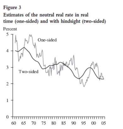
Source: Figure 3 from Tao Wu, “Estimating the ‘Neutral’ Real Interest Rate in Real Time,” Federal Reserve Bank of San Francisco, Economic Letter, No. 2005-27, October 21, 2005.

Source: Figure 3 from Tao Wu, “Estimating the ‘Neutral’ Real Interest Rate in Real Time,” Federal Reserve Bank of San Francisco, Economic Letter, No. 2005-27, October 21, 2005.

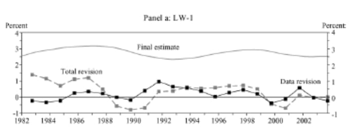
Source: Figure 3 p. 407: Todd E. Clark and Sharon Kozicki, “Estimating Equilibrium Real Interest Rates in Real Time,” North American Journal of Economics and Finance 16, 2005, pp. 395-413.

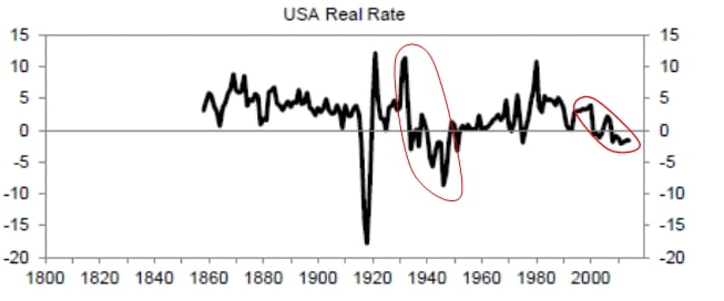
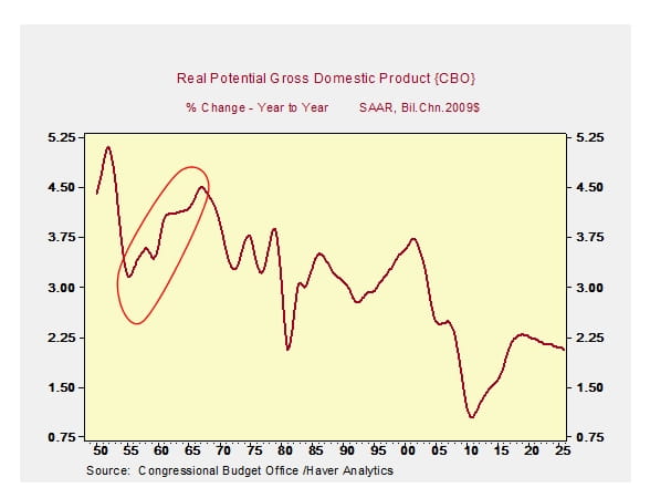
Source: J.D. Hamilton, E.S. Harris, J. Hatzius, and K.D. West, “The Equilibrium Real Funds Rate: Past, Present, and Future,” February 2015.

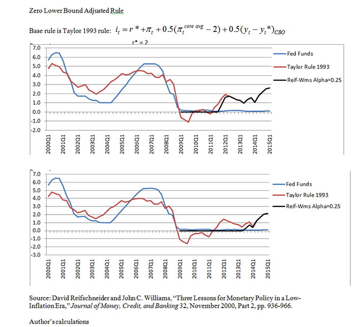
Source: David Reifschneider and John C. Williams, “Three Lessons for Monetary Policy in a Low-Inflation Era,” Journal of Money, Credit, and Banking 32, November 2000, Part 2, pp. 936-966; author's calculations

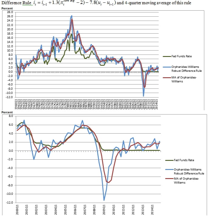
Source: Athanasios Orphanides and John C. Williams, “Robust Monetary Policy Rules with Unknown Natural Rates,” Brookings Papers on Economic Activity 2, 2002, pp. 63-145; author's calculations.

References

- Barsky, Robert, Alejandro Justiniano, and Leonardo Melosi, “The Natural Rate and its Usefulness for Monetary Policy Making,” American Economic Review: Papers and Proceedings 104, May 2014, pp. 37-43.
- Clark, Todd E., and Sharon Kozicki< rel="noopener noreferrer" a="" class="offsite" target="_blank" href="https://ideas.repec.org/p/fip/fedkrw/rwp04-08.html" />, “Estimating Equilibrium Real Interest Rates in Real Time,” North American Journal of Economics and Finance 16, 2005, pp. 395-413.
- Giannoni, Marc P., “Does Model Uncertainty Justify Caution? Robust Optimal Monetary Policy in a Forward-Looking Model,” Macroeconomic Dynamics 6, 2002, pp. 111-141.
- Giannoni, Marc P., “Robust Optimal Monetary Policy in a Forward-Looking Model with Parameter and Shock Uncertainty,” Journal of Applied Econometrics 22, 2007, pp. 179-213.
- Laubach, Thomas, and John C. Williams, “Measuring the Natural Rate of Interest.” Review of Economics and Statistics 85, 2003, pp. 1063-1070.
- Orphanides, Athanasios, and John C. Williams, “Robust Monetary Policy with Imperfect Knowledge,” Journal of Monetary Economics 54, 2007, pp. 1406-1435.
- Orphanides, Athanasios, and John C. Williams, “Robust Monetary Policy Rules with Unknown Natural Rates,” Brookings Papers on Economic Activity 2, 2002, pp. 63-145.
- Reifschneider, David, and John C. Williams, “Three Lessons for Monetary Policy in a Low-Inflation Era,” Journal of Money, Credit, and Banking 32, November 2000, Part 2, pp. 936-966.
- Taylor, John B., “Discretion versus Policy Rules in Practice,” Carnegie-Rochester Conference Series on Public Policy 39, 1993, pp. 195-214.
- Taylor, John B., “A Historical Analysis of Monetary Policy Rules,” in J.B. Taylor, ed., Monetary Policy Rules, Chicago: University of Chicago Press, 1999, pp. 319-341.
- Wicksell, Knut, Interest and Prices, 1898.
- Woodford, Michael, “Methods of Policy Accommodation at the Interest-Rate Lower Bound,” Federal Reserve Bank of Kansas City 2012 Economic Policy Symposium, The Changing Policy Landscape.
- Wu, Tao, “Estimating the ‘Neutral’ Real Interest Rate in Real Time,” Federal Reserve Bank of San Francisco, Economic Letter, No. 2005-27, October 21, 2005.