

- Share
Challenges with Estimating U Star in Real Time
Although the concept of the natural rate of employment, NAIRU, or “U star” is used to measure the amount of slack in the labor market, it is an unobservable quantity that must be estimated using data currently available. This Commentary investigates the degree to which our estimates of U star at various points in the current business cycle have changed as real-time data have been revised and as more data points have accumulated. I find that the availability of additional data has contributed to a significant change in our estimates of U star at earlier points in the business cycle, a result that suggests we might have been underestimating the level of labor market slack during some of the recent recovery period. In retrospect, our updated estimates of U star suggest labor markets were not as tight as we thought they were then.
The views authors express in Economic Commentary are theirs and not necessarily those of the Federal Reserve Bank of Cleveland or the Board of Governors of the Federal Reserve System. The series editor is Tasia Hane. This paper and its data are subject to revision; please visit clevelandfed.org for updates.
Economists measure the degree of labor market slack in the economy by comparing the observed unemployment rate to the rate that would be considered “normal” given other conditions present at the time. This normal rate is referred to variously as the natural rate of unemployment, the nonaccelerating inflation rate of unemployment (NAIRU), or sometimes just U star (or U*). Unfortunately, U* is unobservable and subject to a lot of uncertainty. The uncertainty around this estimate is a well-known problem (Steigler et al., 1997) and it has significant implications for policymakers (Orphanides and Williams, 2002).
Another challenge with using U* to gauge labor market slack has to do with the nature of economic policymaking in real time: Policymakers must base their estimates of U*—and their policy decisions—on data available in the moment, data that are almost always later revised. Revisions reflect the availability of more complete data, methodological improvements, better accounting of seasonal factors, and so forth. Sometimes, just the sheer availability of more data points with the passage of additional time might change what we think about the behavior of a variable of interest.
In this Commentary, I investigate how data revisions and the availability of longer time series have altered our estimates of U* over the past decade. I find that data revisions have not played a big role over this period but the availability of additional data has contributed to a significant change in our estimates of U* at earlier points in the business cycle. The analysis suggests that we might have been underestimating the level of labor market slack during some of the recent recovery period. In retrospect, our updated estimates of U* suggest labor markets were not as tight as we thought they were then.
Alternative Estimates of U*
A number of different approaches to estimating U* exist. I consider four here: (1) a model-based estimate, and the publicly available estimates of (2) the Congressional Budget Office, (3) the Survey of Professional Forecasters, and (4) the Federal Open Market Committee. Note that these sources may call their estimates something other than U*, but I will refer to them all as U* for simplicity.
The model-based estimate of U* follows an approach presented in Tasci (2012) and described nontechnically in Tasci and Zaman (2010). This approach looks at trends in labor market flows and is informed by the modern search theory of unemployment. It recognizes that the unemployment rate depends on underlying flows of workers moving into and out of unemployment. These underlying flow rates have significant cyclical components along with a trend component that could be due to demographics or other factors.The basic idea of this approach is to estimate a statistical model that will tease out the cyclical component from the underlying trend. Once we obtain trend estimates from the flow rates, we can use the estimated trend levels to compute a long-run rate that is consistent with the search theory of unemployment.
In practice, when trying to disentangle cyclical movements from the trend in labor market variables, we rely on the cyclical movements in real output. The cyclical component in each of the flow rates is identified by its comovement with respect to the cyclical component of real output. This method allows us to estimate U* with just three observable variables: real output, the rate of flow into unemployment (the separation rate), and the rate of flow out of unemployment (the job-finding rate). In the rest of the text, I will refer to this estimate of U* as the flow-model estimate.
The Congressional Budget Office’s (CBO) estimate of U* is usually released twice per year, once in the first quarter and again in the third quarter. The CBO relies on a set of statistical models to estimate the level of potential output and potential labor input over time. It defines its U* estimate as “the rate that arises from all sources other than fluctuations in demand associated with business cycles.”1
Another estimate of U* comes from the Survey of Professional Forecasters (SPF), a quarterly survey of forecasters from the private sector and academia that is conducted by the Federal Reserve Bank of Philadelphia. In the third quarter of every year, survey participants are asked to provide their estimates of U*.2 For the SPF estimate of U*, I use the median projection of the forecasters.
One other estimate of U* is obtainable from the projections of Federal Open Market Committee (FOMC) participants. Four times a year, FOMC participants provide their projections, referred to as the Summary of Economic Projections (SEP). One of these variables is the unemployment rate in the long run. These longer-run projections are defined as “… the rates of growth, unemployment and inflation to which a policymaker expects the economy to converge over time—maybe in five or six years—in the absence of further shocks and under appropriate monetary policy.3 ” This long-run projection for the unemployment rate is in part similar to the flow-model estimate since it abstracts from further shocks, including cyclical movements. On the other hand, the flow-model estimate does not make any assumptions about the stance of monetary policy whereas the SEP estimates do. For the SEP estimate of U*, I use the median projection of the FOMC participants.
Note that the SPF and SEP estimates are real-time assessments of U* by participants in the respective surveys. In these surveys, this amounts to participants’ best forward-looking judgment about U* with the data available to them at the time. However, these surveys do not provide U* estimates for a period in the past retrospectively. By contrast, the CBO updates its past projections and provides these in every release along with the whole history of its U* estimates. Hence, the real-time estimate for 2010, for instance, could conceivably be different from the estimate for 2010 in the most recent vintage. Similarly, the flow-model estimate in real-time could be different from the most recent estimate because as the underlying data are revised, the estimation potentially delivers a new set of parameter estimates. Therefore, to assess whether data revisions and the availability of longer time series have altered our estimates of U* over the past decade, I compare the real-time and last-period estimates of the CBO and the flow-model. The SPF and SEP estimates are included to provide additional context in real time.
Comparing Estimates of U*
I first compare the real-time estimates of U* that were made over the course of the past recession and recovery from each of the four sources. Then I compare those estimates with the latest estimates of U* for that period from the CBO and the flow model.
Real-time Estimates of U*
Real-time estimates of U* were relatively close to each other during the past recession (figure 1). When the prior expansion ended in 2007:Q4, the unemployment rate was 4.8 percent, slightly above the expansion’s low of 4.5 percent. In the same period, U* estimates ranged from 4.5 percent (flow model) to 4.8 percent (CBO), with the SPF right in the middle at 4.65 percent.4 By the end of the recession in 2009:Q2, the unemployment rate had hit 9.3 percent. Despite this large increase, estimates of U* remained within a narrow band, between 4.8 percent (CBO) and 5.1 percent (flow model). This is not surprising, as U* estimates, despite their varying definitions, aim to see through cyclical shocks. Hence, the stability of these estimates suggests that neither the statistical model nor professional forecasters interpreted the sharp increase in the unemployment rate as indicative of a permanent and substantial shift in U*.
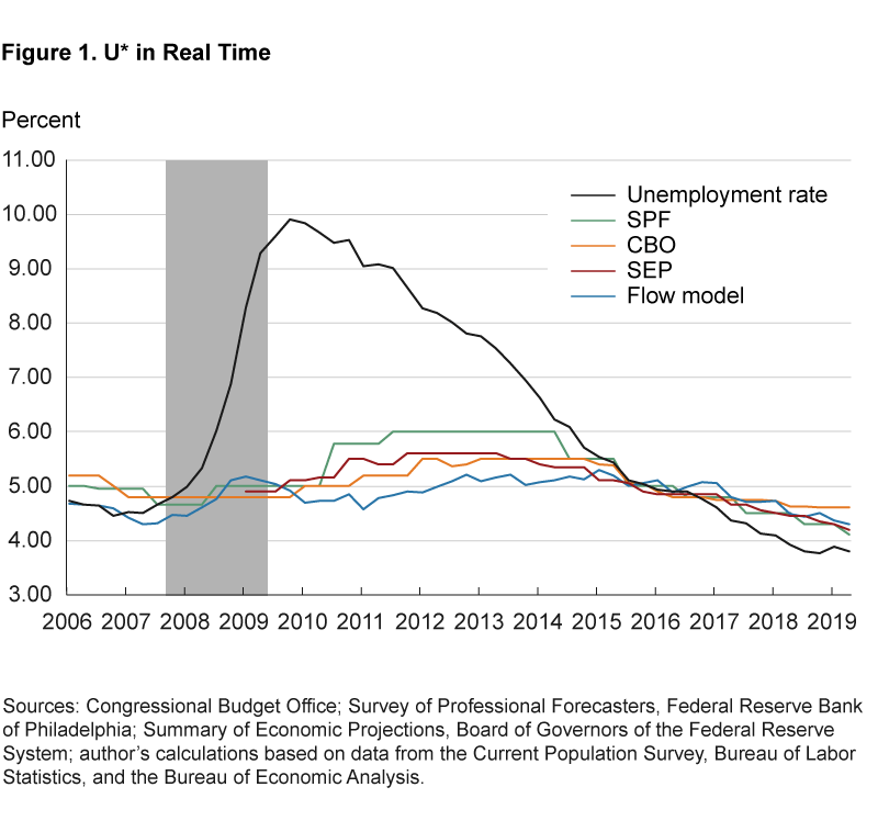
However, real-time estimates of U* started to diverge from each other starting in 2010. Even though the flow-model’s estimate stayed somewhat stable and low, the SPF’s and SEP’s ticked up slightly. At some point in early 2011, the difference between the SPF forecast for U* and the flow-model’s estimate stood at 1.2 percentage points, about one-fifth of the average unemployment rate in the United States. Therefore, if we were to judge the extent of labor market slack around that time, we would have come up with different answers depending on which U* estimate we used.
Current Estimates of Historical U*
We next analyze how much the real-time estimates differ from our current “best” estimates, comparing real-time estimates of period-t with current estimates of period-t, n-periods later at t+n. As noted above, current estimates of past U* values are available for only the CBO and flow-model estimates. Figure 2 shows the real-time and current estimates of U* from these two sources. Several interesting patterns emerge from this picture.
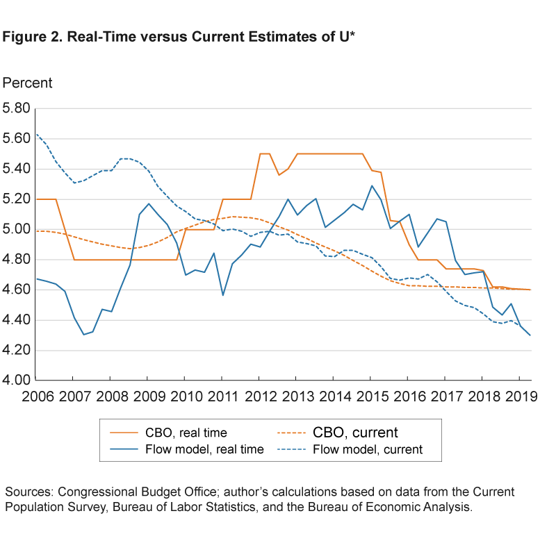
First, current vintages of the flow-based and CBO estimates of U* are a lot closer to each other than are the corresponding real-time estimates. In fact, between 2010 and 2017 they are virtually indistinguishable. Second, current estimates of U* from both sources are significantly different from their real-time counterparts. For the flow-model, the differences appear during the prerecession period, with estimates for that period much higher now (above 5 percent) than they were in real time (below5 percent). For the CBO, the differences appear during a substantial portion of the recovery, with real-time estimates of around 5.5 percent from 2011 through 2015 and current estimates revised down toward the 5 percent neighborhood. We can conclude that the flow-model estimates of U*, in real time, would have led us to overestimate labor market slack prior to the recession,5 whereas U* estimates from both sources would have led us to underestimate it for a period during the recovery.
Reasons for the Differences over Time
I explore two possible reasons for the significant divergence of real-time U* estimates from their current vintages: revised data and new data. Various data series are used to calculate U* for the CBO and the flow model, and any of these may be revised after their initial release and alter our past estimates of U*. And, over time, as new data points become available for these series, our interpretation of their trajectories could change and alter those past estimates of U*.
Revised Data
The CBO’s estimate of U* relies on estimates of potential output growth from its forecasting model and demographic and labor market data obtained from the Bureau of Labor Statistic’s household survey.6 Similarly, the flow model relies on estimates of the current level of output and labor market flows estimated from the household survey. It is safe to assume that revisions in the household survey data did not play a significant role because those data are rarely significantly revised, with the exception of seasonal adjustments and benchmarking for population adjustments.
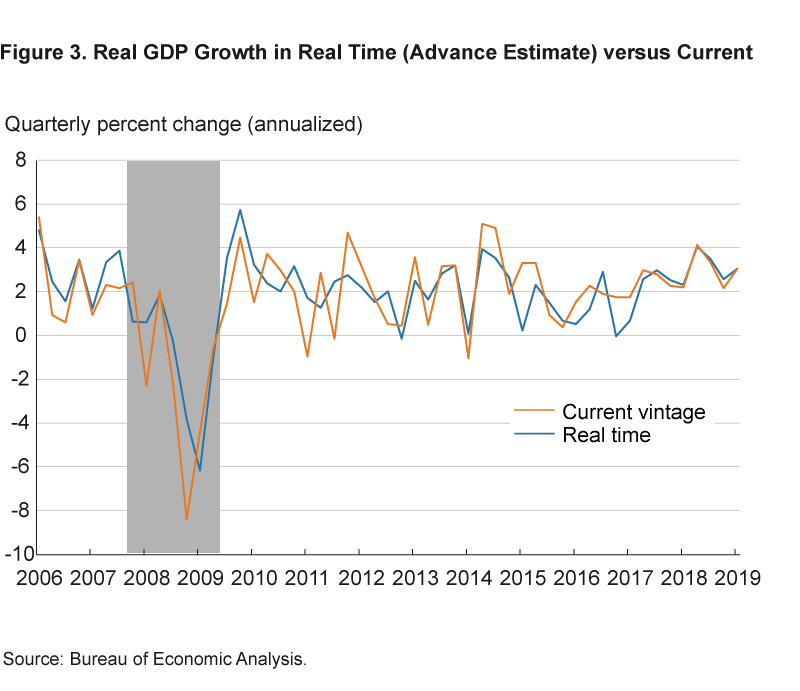
One data source that is used in both the CBO and flow-model approaches is real GDP data. The Bureau of Economic Analysis (BEA) regularly revises GDP estimates as more complete data become available. The first release of the estimate for a particular quarter (advance estimate) is usually published at the end of the first month in the following quarter. The second and third estimates update the advance estimate with more complete and detailed data and are usually released at the end of the second and third months of the quarter following the reference one. More importantly, the BEA implements annual and comprehensive data revisions with newly available major source data and methodological improvements.7 According to the BEA’s own analysis, the average revision to the quarterly percent change in real GDP between the advance estimate and the third estimate is about 0.6 percentage points (at annual rates), without regard to sign. Over longer time periods, revisions could be as large as 1.2 percentage points on average.
Figure 3 compares the real-time quarterly growth rate of real GDP with the current vintage since 2006. Even though there are differences between the two vintages, they are slight. The average revision between the advance estimate (real-time measure) and the final estimate since 2006 is 1.1 percentage points, not necessarily different from the average reported by the BEA for a longer sample period. At least for the flow model, we know that such a difference between the real-time and final vintage for real GDP does not account for the shift in the U* estimates over time.8
New Data
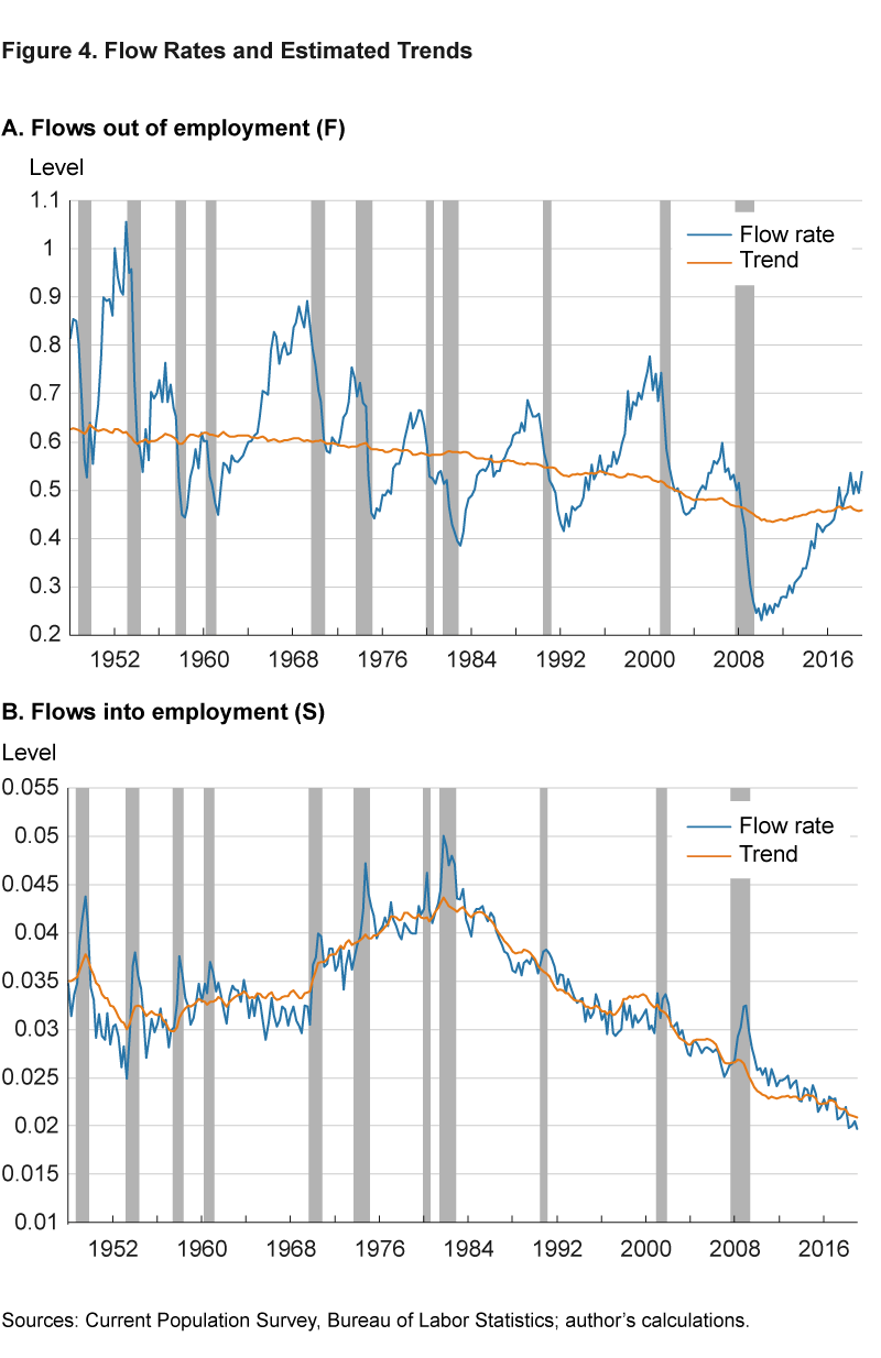
The final possibility for revisions to U* estimates over time is the availability of a longer history of the data series used to calculate U*. We can analyze this possibility for the flow-model very easily. Recall that in addition to the GDP data, there are two additional sources of inputs to the flow model: flows out of unemployment (the job-finding rate) and flows into unemployment (the separation rate).
Figure 4 presents these inputs for the model and the current estimated trends. Since the U* estimate of the flow-model depends on the trend estimates of these flow rates, changes in the estimated trends map into shifts in the implied U* estimate.9
What stands out in figure 4 is the extent of the decline in the job-finding rate depicted on the left panel. Not only was it one of the largest drops in the available data, it also dropped to its lowest level ever by the end of the last recession. It is not uncommon for this flow rate to decline sharply during a recession, but the lowest level reached following the last recession (0.22) was almost 50 percent lower than the previous historical low (0.39) in 1982. Moreover, it stayed below that previous low until 2014. This unprecedented level and the slow recovery afterward led to trend estimates for this flow rate to identify a sharply declining trend in the aftermath of the recession and a relatively stable (almost flat) trend prior to it. In retrospect, the current estimated trend ended up between those extremes. Since a higher trend estimate for this flow rate pushes U* down in real time and a lower trend estimate pushes it up, U* was lower prior to the recession and higher afterward relative to the current estimate.10
Conclusion
It is not easy to gauge how much slack there is in the labor market. Alternative estimates of U* provide a menu of potentially useful benchmarks. However, estimating U* in real time is even more challenging. This analysis has shown that current estimates of U* for the past recession and current recovery differ significantly from estimates made using real-time data. Such differences could arise either from subsequent revisions to the real-time data that are used to calculate U* or as more data accrues over time (which could affect the estimates of trend measures used to calculate U*). I find that the latter is responsible for the time period analyzed. Specifically, we did not know until recently how exceptionally low the job-finding rate would be now. This analysis suggests that we might have been underestimating the level of labor market slack during some of the recent recovery period. In retrospect, both the CBO and flow-model estimates of U* are lower than the real-time estimates, suggesting labor markets were not as tight as we thought they were then.
Footnotes
- For a more detailed description of the model, please see Shackleton (2018).Return
- Note that, the SPF does not provide any information about how individual forecasters come up with their forecasts. Return
- See the June 2019 press release on projection materials for more details on this issue: https://www.federalreserve.gov/monetarypolicy/fomcprojtabl20190619.htm Return
- The first SEP submission is for 2009:Q1. Return
- Based on its own current vintage estimates. Return
- For a more detailed description of the model, please see Shackleton (2018).Return
- For a detailed description of the different forms of revisions, see for instance, the BEA’s recent data release at https://www.bea.gov/system/files/2019-08/gdp2q19_2nd_0.pdf Return
- We have checked this by estimating the path for U* using different vintages of GDP data. Return
- Note that there is virtually no difference between the real-time estimates of these flow rates and the current vintages. Return
- In order to see this, consider the definition U*= S/(F+S), where F and S correspond to job-finding and separation rate trends, respectively. Hence, a higher F pushes U* down.Return
References
- Orphanides, Athanasios, and John C. Williams. 2002. “Robust Monetary Policy Rules with Unknown Natural Rates.” Brookings Papers on Economic Activity, 2002-2.
- Shackleton, Robert. 2018. “Estimating and Projecting Potential Output Using CBO’s Forecasting Growth Model.” Congressional Budget Office, Working Paper 2018-03.
- Staiger, Douglas, James H. Stock, and Mark W. Watson. 1997. “How Precise Are the Estimates of the Natural Rate of Unemployment?” In Romer, C. and D. Romer (eds.), Reducing Inflation: Motivation and Strategy, University of Chicago Press, pp. 195–242.
- Tasci, Murat. 2012. “The Ins and Outs of Unemployment in the Long Run: Unemployment Flows and the Natural Rate.” Federal Reserve Bank of Cleveland, Working Paper, No 12-24.
- Tasci, Murat, and Randal Verbrugge. 2014. “How Much Slack Is in the Labor Market? That Depends on What You Mean by Slack.” Federal Reserve Bank of Cleveland, Economic Commentary, 2014-21.
- Tasci, Murat, and Saeed Zaman. 2010. “Unemployment after the Recession: A New Natural Rate?” Federal Reserve Bank of Cleveland, Economic Commentary, 2010-11.
Suggested Citation
Tasci, Murat. 2019. “Challenges with Estimating U Star in Real Time.” Federal Reserve Bank of Cleveland, Economic Commentary 2019-18. https://doi.org/10.26509/frbc-ec-201918
This work by Federal Reserve Bank of Cleveland is licensed under Creative Commons Attribution-NonCommercial 4.0 International

