

- Share
The Likelihood of 2 Percent Inflation in the Next Three Years
This Commentary examines inflation forecasts generated from a range of statistical models that historically have performed well at forecasting inflation. For each model, we look at the most likely future forecast path and the distribution of forecasts around that path. We show that the models project generally rising inflation, but, in contrast to other forecasts, five out of six models assign a less than 50 percent probability to inflation’s being 2 percent or higher over the next three years.


The views authors express in Economic Commentary are theirs and not necessarily those of the Federal Reserve Bank of Cleveland or the Board of Governors of the Federal Reserve System. The series editor is Tasia Hane. This paper and its data are subject to revision; please visit clevelandfed.org for updates.
Over most of the last five years, inflation as measured by the price index for personal consumption expenditures (PCE) has been less than 2 percent. Many forecasters during this time expected that inflation would turn up, only to be repeatedly surprised. Recent forecasts from professional economists again have inflation rising to 2 percent over the next two to three years. What is the likelihood that such a forecast will come to pass?
To answer this question, this Commentary examines the inflation forecasts coming from a range of statistical models that historically have performed well in forecasting inflation, and it shows both the point forecasts and the densities, or probabilities, around those forecasts.
In five of the six models we consider, the probability that inflation will be at least 2 percent over the next three years is less than 50 percent. Specifically, the estimated likelihood that PCE inflation will be at least 2 percent ranges from 11 percent to 49 percent by the end of 2017, 16 percent to 51 percent by the end of 2018, and 18 percent to 49 percent by the end of 2019. These results vary widely, but because all six models demonstrate comparable historical forecasting accuracy, we cannot adjudicate between these competing models and forecasts.
Recent Inflation Data and Forecasts
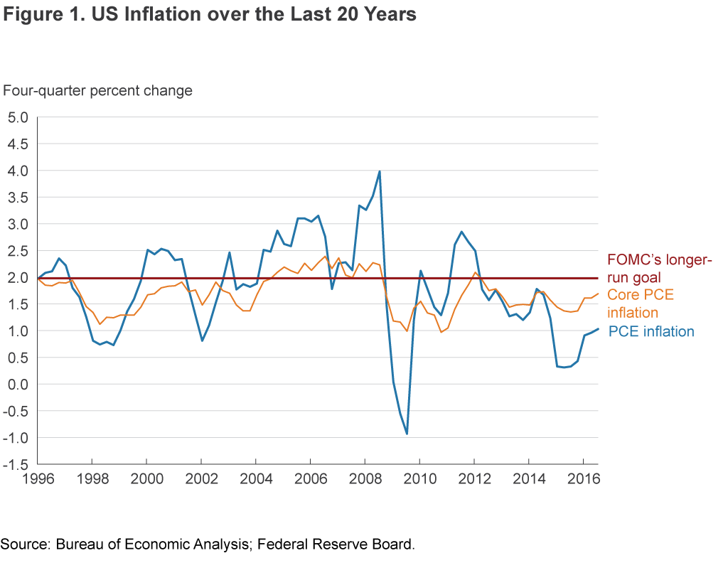
Inflation as measured by the PCE has averaged 1.4 percent on a trailing four-quarter basis since the recovery began in 2009:Q3—0.6 percentage points below the Federal Open Market Committee’s (FOMC) long-run objective of 2 percent. By comparison, over the 10-year period preceding the financial crisis, PCE inflation averaged 2.0 percent (see figure 1). Meanwhile, inflation excluding food and energy (core PCE) averaged 1.5 percent and 1.8 percent over the same periods, respectively.
Not only has PCE inflation been below 2 percent for most of the recent past, it has also persistently come in below many economists’ forecasts. For example, in 2013:Q1, the median forecast from the Survey of Professional Forecasters (SPF) was 2.0 percent for 2014:Q4 and 2015:Q4, whereas actual inflation turned out to be 1.2 percent and 0.4 percent, respectively. Similarly, the median forecast for core inflation was 1.9 percent for both 2014 and 2015, while actual core inflation was 1.6 percent and 1.4 percent, respectively. Projections made by FOMC participants around the same time display similar forecast misses.
Looking ahead, most forecasts again call for inflation to rise toward 2 percent. At the September 2016 FOMC meeting, the median projection in the FOMC’s Summary of Economic Projections (SEP) for PCE inflation was 1.9 percent for 2017:Q4 and 2.0 percent for both 2018:Q4 and 2019:Q4. For core PCE, the median projections were 1.8 percent, 2.0 percent, and 2.0 percent, respectively. Projections from the 2016:Q4 SPF were similar, with the median forecasts for PCE inflation rising from 1.9 percent in 2017:Q4 to 2.0 percent in 2018:Q4, and for core PCE inflation rising to 1.9 percent in 2017:Q4 and remaining flat through 2018:Q4.
Comparisons with Statistical Forecasting Models
The inflation forecasts of economists and policymakers are often informed by statistical models. While there is no agreement on a single “best” model for the inflation process, we chose for our analysis six statistical models that have been shown to forecast inflation well over the medium term (i.e., two to three years); this forecasting horizon seems to be the most appropriate for monetary policy.1
To improve forecasting accuracy, the models we consider include stochastic volatility, or a time-varying standard deviation of the size of the shocks hitting the economy. An increasing body of research has shown that incorporating stochastic volatility into macroeconomic models improves the precision of both point and density forecasts of inflation.2
All the models are estimated with quarterly data through 2016:Q3.3 We run these six models twice: The first run uses PCE inflation as our inflation variable, the second uses core PCE inflation. This allows us to generate an outlook for both of these inflation indicators.4
Our first model is the univariate unobserved components model of Stock and Watson (2007). This model assumes that at any point in time inflation (headline or core) is the sum of two underlying unobservable components: trend inflation and temporary fluctuation around this trend. The trend component follows a random walk process, which varies over time in response to unexpected shocks. The standard deviation of the size of these unexpected shocks is allowed to vary over time. The other component, the temporary deviation from the trend, is assumed to be serially uncorrelated. The standard deviation of the shocks that are responsible for these transitory deviations also varies over time. The model uses inflation’s own history to estimate the two components. The estimated value of the trend component at each point in time is the point forecast of inflation far into the future, implying a perfectly flat path for the point forecast. One notable property of this forecasting model is that the estimated trend can be influenced by a persistent sequence of observations that the model interprets as resulting from a change in the underlying trend. One period’s blip up or down can be perceived as “noise,” whereas a sequence of higher inflation rates can alter the estimate of the trend. We denote this model UCSV.
Our second model is a bivariate unobserved components model as in Chan, Clark, and Koop (2015). This model is an extension of the Stock and Watson (2007) univariate UCSV model as it uses both inflation’s own history and the data from long-run inflation expectations to estimate trend inflation.5 The model allows for time-variation in the relationship between trend inflation and the long-run forecast of inflation in addition to stochastic volatility. We denote this model TVP-Bi-UCSV.
Our third model is the unobserved components model as in Tallman and Zaman (forthcoming). This model exploits a Phillips-curve relationship that may be relevant for some inflation subaggregates but not others. Specifically, forecasts of aggregate inflation are produced by separately forecasting services inflation and goods inflation, using two different models, and then aggregating the forecasts.6 The model used to forecast services inflation is a bivariate unobserved components model that exploits the Phillips curve relationship between services inflation and the unemployment rate. The model for goods inflation is a univariate UCSV model as in Stock and Watson (2007) but applied to goods inflation. We denote this model Services and Goods UCSV.7
Our fourth model closely follows the model laid out in Clark (2011). The model is a small-scale vector autoregression estimated using Bayesian methods and a steady-state prior. The model consists of the following four variables: the unemployment rate, real GDP growth, the federal funds rate, and PCE inflation (or core PCE inflation).8 Both the inflation rate and the unemployment rate enter the model as deviations from their respective trends (i.e., gaps), where the trends are taken from external sources.9 In this model, the equation for the inflation gap is a function of its own lags and the lags of other variables including the unemployment gap. The advantage of modeling inflation this way—that is, as a gap—is that inflation forecasts in the medium- to long-term remain anchored around the exogenous trend rate. Research has shown that this method helps improve inflation forecast accuracy. We denote this model SS-SV-BVAR.
Our fifth model is a time-varying parameter vector autoregression as in D’Agostino et al. (2013).10 This model has three variables: the unemployment rate, the federal funds rate, and inflation. As the name suggests, it allows for the possibility of changing relationships among the economic variables of interest over time in addition to changing volatility of the shocks hitting the economy. Inflation in this model at any point in time is a function of its own lags and the lags of the other variables. We denote this model TVP-SV-BVAR.
Finally, our sixth model is an autoregressive (AR) gap model similar to that of Faust and Wright (2013) but augmented to allow stochastic volatility as detailed in Chan, Clark, and Koop (2015). Specifically, inflation is modeled as the deviation from long-run inflation expectations (denoted as the inflation gap), which is assumed to follow an autoregressive process with a single lag. We denote this model AR1-SV-Gap.
Point Forecasts
Each of these six models is estimated using data through 2016:Q3 and then simulated to obtain thousands of forecast paths up to 13 quarters out in order to match the SEP projection horizon (i.e., from 2016:Q4 to 2019:Q4).11 The mean of these thousands of forecast paths is denoted as the point forecast; it reflects the most likely forecast of future inflation generated by a given model.12
Table 1 reports the point forecasts for four-quarter trailing inflation rates at three set of dates from our set of six models. It also reports the simple arithmetic average of the forecasts from the six models. Forecasts from the SPF and the FOMC SEP are provided for comparison. The three representative dates match the forecast dates reported in the SEP and SPF.
| PCE inflation | 2017:Q4 | 2018:Q4 | 2019:Q4 |
|---|---|---|---|
| UCSV | 1.1 | 1.1 | 1.1 |
| TVP-Bi-UCSV | 1.7 | 1.7 | 1.7 |
| Services and Goods UCSV | 1.2 | 1.1 | 1.1 |
| SS-SV-BVAR | 2.0 | 2.1 | 2.0 |
| TVP-SV-BVAR | 1.7 | 1.8 | 1.9 |
| AR1-SV-Gap | 1.9 | 1.9 | 1.8 |
| Average of above models | 1.6 | 1.6 | 1.6 |
| SPF (median) | 1.9 | 2.0 | n.a. |
| FOMC SEP (median) | 1.9 | 2.0 | 2.0 |
| Core PCE inflation | |||
| UCSV | 1.7 | 1.7 | 1.7 |
| TVP-Bi-UCSV | 1.6 | 1.6 | 1.6 |
| Services and Goods UCSV | 1.7 | 1.6 | 1.6 |
| SS-SV-BVAR | 1.8 | 1.8 | 1.8 |
| TVP-SV-BVAR | 1.7 | 1.6 | 1.6 |
| AR1-SV-Gap | 1.8 | 1.8 | 1.8 |
| Average of above models | 1.7 | 1.7 | 1.7 |
| SPF (median) | 1.9 | 1.9 | n.a. |
| FOMC SEP (median) | 1.8 | 2.0 | 2.0 |
Notes: All numbers show four-quarter inflation rates. Model forecasts use data through 2016:Q3. The SPF (median) corresponds to the 2016:Q4 Survey of Professional Forecasters. The FOMC SEP (median) corresponds to the September 2016 Summary of Economic Projections.
The point forecasts for PCE inflation over the next three years display notable differences across the models. For example, for 2017:Q4 (as well as for 2019:Q4) inflation projections range anywhere from 1.0 percent to 2.0 percent.
For context, the first three models under consideration belong to the class of models called the “unobserved components” model. In these models, the inflation forecast is driven mainly by the value of the inflation trend component estimated at the time the forecast is made. The UCSV model assumes that the “point” forecast of inflation arbitrarily far into the future is the current estimate of the trend inflation. Given that inflation has been relatively low for a while, both the UCSV model and the Services and Goods UCSV model estimate a low level of trend inflation and hence forecast low future inflation. In the TVP-Bi-UCSV, the inclusion of inflation expectations that are stable at 2 percent strongly influences the estimate of trend inflation.
The remaining three models belong to the class of vector autoregressive models (VARs); forecasts from VARs are essentially glide paths that begin from the recent actual value of a variable and converge to these models’ own estimates of the variable’s (in our case inflation’s) long-run value.13 In two of the three models, the long-run inflation rate or trend rate comes from outside the model instead of being estimated, and with that trend currently at 2 percent, these two models return closer to 2 percent in the medium to long term.14 The forecasts from these three models are all generally higher than those coming from the first three models: 1.7 percent to 2.0 percent for 2017:Q4, 1.8 percent to 2.1 percent for 2018:Q4, and 1.8 percent to 2.0 percent for 2019:Q4. They are also within the range of the FOMC projections reported in the September SEP (see table 1).
The forecasting literature has shown that historically these six models have delivered comparable forecast accuracy. Given this competitiveness, all the information in these models’ forecasts can be combined and used at the same time by averaging them into a single forecast. When each forecasting model’s prediction is equally weighted, the resulting forecast is low—PCE inflation is projected to be 1.6 percent over the next three years (table 1). That forecast is about four-tenths lower than the SEP’s median projection.
For core PCE inflation, the models’ combined forecast for inflation is 1.7 percent for the next three years, roughly three-tenths lower than the median SEP projection value.
Density Forecasts and Quantifying the Likelihood of Inflation Crossing 2 Percent
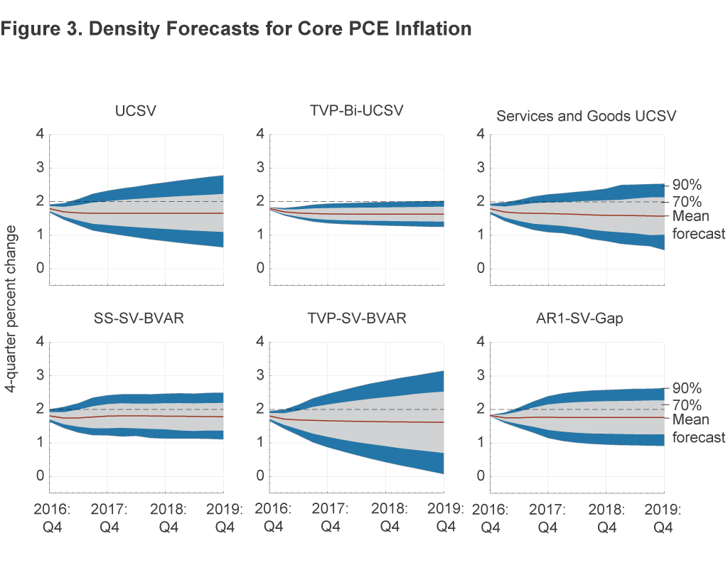
Figure 2 presents the point (mean) forecasts of PCE inflation along with the 70 percent and 90 percent probability bands around them. Figure 3 does the same for core PCE inflation. The figures show the FOMC’s long-run inflation goal of 2 percent to give a visual sense of where it lies in the probability interval. We make three observations.
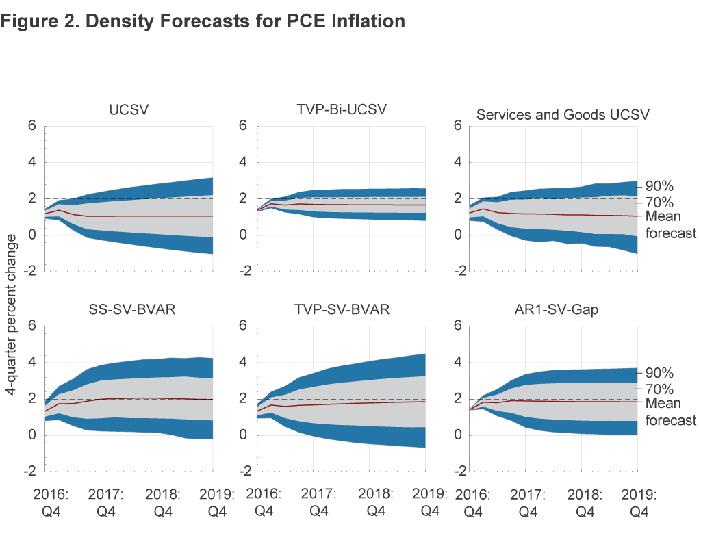
First, each forecast entails considerable uncertainty. Based on data through 2016:Q3, the narrowest forecast probability bands are associated with the TVP-Bi-UCSV model, whereas TVP-SV-BVAR has the widest probability bands.
Second, half of the forecasts for PCE inflation assign a small probability to the prospect of returning to 2 percent. Among the forecasts from the first three models, the line at 2 percent is either outside or just barely touching the 70 percent probability bands. Forecasts from all three of these models would put the odds of inflation’s being greater than or equal to 2 percent at less than 25 percent (table 2).15
| PCE inflation | 2017:Q4 | 2018:Q4 | 2019:Q4 |
|---|---|---|---|
| UCSV | 10.6 | 15.6 | 18.9 |
| TVP-Bi-UCSV | 19.7 | 19.7 | 20.8 |
| Services and Goods UCSV | 14.0 | 17.3 | 17.5 |
| SS-SV-BVAR | 48.9 | 50.7 | 48.5 |
| TVP-SV-BVAR | 35.6 | 42.0 | 44.9 |
| AR1-SV-Gap | 44.7 | 43.9 | 42.9 |
| Core PCE inflation | |||
| UCSV | 15.6 | 21.1 | 23.8 |
| TVP-Bi-UCSV | 3.2 | 4.7 | 5.8 |
| Services and Goods UCSV | 13.1 | 17.7 | 20.5 |
| SS-SV-BVAR | 26.5 | 29.2 | 26.5 |
| TVP-SV-BVAR | 22.7 | 29.4 | 32.9 |
| AR1-SV-Gap | 25.4 | 29.4 | 29.7 |
Notes: Inflation refers to four-quarter trailing inflation. The numbers reported are percentages (probabilities).
However, the remaining three models are somewhat more sanguine about the inflation outlook. In these cases, the2 percent line is inside the 70 percent probability band and closer to the point forecast, suggesting a greater likelihood when compared with the forecasts from models one through three that inflation will exceed or equal 2 percent. The SS-SV-BVAR model forecasts a slightly greater than 50 percent probability that inflation will be 2 percent or higher, a probability which is consistent with that model’s point forecasts of 2.0 percent to 2.1 percent reported in table 1. However, the probabilities in the other two models are less than 50 percent throughout the forecast horizon. Thus, five of the six models considered here place a less than 50 percent probability on PCE inflation’s rising above 2 percent. For core PCE inflation, all six models place a less than 50 percent probability on such an outcome.
Conclusion
Inflation has been running at low levels for most of the past five years and has failed to move higher as expected. This Commentary assesses the likelihood that inflation will increase to at least 2 percent over the next three years by using six forecasting models that research has shown to be accurate for forecasting inflation. For PCE inflation, five of the six models suggest that there is a less than 50 percent probability that inflation will be greater than or equal to 2 percent in the next three years. For core PCE inflation, all six models currently estimate a less than 50 percent probability that inflation will be greater than or equal to 2 percent.
In all of our model simulations, there are wide probability bands around the forecasts, indicating a considerable degree of uncertainty. Inflation in the future could rise above the forecasts, and if the increase were persistent—that is, inflation surprises to the upside—then these inflation observations would likely alter the forecasts as well as the related likelihoods to the upside.
Footnotes
- The forecasting superiority of these models is documented in the following recent studies: Clark, 2011; Faust and Wright, 2013; Clark and Doh, 2014, Chan, Clark, and Koop, 2015; and Tallman and Zaman, forthcoming. Return to 1
- See Stock and Watson, 2007; Clark, 2011; D’Agostino et al., 2013; and Tallman and Zaman, forthcoming. To get a sense of how forecast uncertainty differs between models with and without time-varying volatility see Knotek et al., 2015, who look at the evolution of inflation forecast uncertainty across a variety of models including some with and without time-varying volatility. Three of the models used in this analysis were also used in that study. Return to 2
- The start date of the estimation varies by model. We keep the same start date as it was set in the cited studies; see footnote 11 for details. In principle, we could augment the models with inflation nowcasts for Q4 using the inflation nowcasting model of Knotek and Zaman (forthcoming), but given that the models’ Q4 forecasts of core inflation are identical to the nowcasts and similar for PCE inflation, the models’ forecasts would not be changed materially. Return to 3
- We model these two inflation rates separately to be consistent with the cited studies that estimate models using only one inflation indicator at a time. Return to 4
- The long-run inflation expectations come from the Survey of Professional Forecasters (SPF). Return to 5
- The forecasts of the two components are combined into the forecast for aggregate inflation using the real-time component weights available as of the forecast date. The weights are the relative share of services inflation and goods inflation in overall PCE inflation. The weight for services inflation is computed as the nominal share of personal consumption expenditures of services divided by nominal PCE, and the weight for goods inflation is one minus the services’ share. As of 2016:Q3, goods inflation was assigned a weight of 32 percent and services inflation 68 percent; similarly, core goods’ share was 26 percent and core services’ share 74 percent. Return to 6
- Specifically, goods inflation is decomposed into a random walk trend component and serially uncorrelated transitory component, both of whose variances are allowed to vary over time. Return to 7
- For this analysis, we imposed the following steady states: real GDP growth of 2.0 percent; nominal federal funds rate of 3.25 percent; inflation of 2.0 percent; and an unemployment rate of 5.0 percent. Return to 8
- Specifically, the unemployment rate trend comes from the natural rate series available from the Congressional Budget Office (CBO), and the inflation trend comes from the long-run inflation expectations from the Federal Reserve Board’s econometric model. This series is nicknamed “PTR.” It is a construct based on estimates from Kozicki and Tinsley (2001) and 10-year forecasts from the SPF. Return to 9
- This time-varying parameter model was originally developed by Cogley and Sargent (2005) and Primiceri (2005). D’Agostino et al. (2013) use this model to document its superior forecasting capability especially for inflation against a constant parameter BVAR and other univariate benchmarks. Return to 10
- The UCSV, TVP-Bi-UCSV, and AR1-SV-Gap are estimated with data beginning 1959:Q2; the Services and Goods UCSV is estimated with data beginning 1960:Q1; the SS-SV-BVAR is estimated with data beginning 1985:Q1; and TVP-SV-BVAR is estimated with data beginning 1959:Q2, with the first 10 years used as the training sample for determining the priors. Return to 11
- The simulated paths reflect both shock and parameter uncertainty. Parameter uncertainty is accounted for by drawing different a set of parameters for each simulated path. Shock uncertainty is reflected by drawing a set of shocks specific to the model’s estimation of historical data. Return to 12
- The estimated (unrestricted) long-run values for the variables in the VAR are the unconditional sample mean of the variable. Therefore, the model’s estimated long-run value will depend on the sample period used for estimation. In our steady-state BVAR, a long-run value for inflation of 2 percent is imposed; as a result, this model goes toward 2 percent very quickly. This model is called a steady-state BVAR because we could choose to impose long-run values on any or all of the variables that comprise it. Return to 13
- The models do not necessarily converge precisely to 2 percent because the presence of a constant term in the inflation gap equation captures the long-run historical deviation of the inflation gap from zero within the estimation sample. The estimated value of the constant term will be positive if inflation has exceeded the inflation trend on average during the sample, while it will be negative if inflation has been below trend on average. Return to 14
- These likelihoods reflect the probability, computed as the fraction of the simulations, that inflation is greater than or equal to 2 percent at those specific dates. Return to 15
References
- Chan, Joshua C.C., Todd E. Clark, and Gary Koop, 2015. “A New Model of Inflation, Trend Inflation, and Long-Run Inflation Expectations,” Federal Reserve Bank of Cleveland, Working Paper no. 15-20.
- Clark, Todd E., and Taeyoung Doh, 2014. “Evaluating Alternative Models of Trend Inflation,” International Journal of Forecasting, 30: 426–448.
- Clark, Todd E., 2011. “Real-Time Density Forecasts from Bayesian Vector Autoregressions with Stochastic Volatility,” Journal of Business and Economic Statistics, 29(3): 327–41.
- Cogley, Timothy, and Thomas J. Sargent, 2005. “Drifts and Volatilities: Monetary Policies and Outcomes in the Post WWII U.S.” Review of Economic Dynamics, 8: 262–302.
- D’Agostino, Antonello, Luca Gambetti, and Domenico Giannone, 2013. “Macroeconomic Forecasting and Structural Change,” Journal of Applied Econometrics, 28(1): 82–101.
- Faust, Jon, and Jonathan H. Wright, 2013. “Forecasting Inflation,” in Graham Elliott and Allan Timmermann, eds., Handbook of Economic Forecasting, vol. 2, Elsevier: North Holland.
- Knotek II, Edward S., Saeed Zaman, and Todd E. Clark, 2015. “Measuring Inflation Forecast Uncertainty,” Federal Reserve Bank of Cleveland, Economic Commentary, no. 2015-03.
- Knotek II, Edward S., and Saeed Zaman, forthcoming. “Nowcasting U.S. Headline and Core Inflation,” Journal of Money, Credit and Banking.
- Kozicki, Sharon, and P.A. Tinsley, 2001. “Shifting Endpoints in the Term Structure of Interest Rates,” Journal of Monetary Economics, 47(3): 613–52.
- Primiceri, Giorgio, 2005. “Time Varying Structural Vector Autoregressions and Monetary Policy” Review of Economic Studies, 72: 821–852.
- Stock, James H. and Mark W. Watson, 2007. “Why Has U.S. Inflation Become Harder to Forecast?” Journal of Money, Credit and Banking, 39(S1): 3–33.
- Tallman, Ellis, and Saeed Zaman, forthcoming. “Forecasting Inflation: Phillips Curve Effects on Services Price Measures,” International Journal of Forecasting.
Suggested Citation
Tallman, Ellis W., and Saeed Zaman. 2016. “The Likelihood of 2 Percent Inflation in the Next Three Years.” Federal Reserve Bank of Cleveland, Economic Commentary 2016-14. https://doi.org/10.26509/frbc-ec-201614
This work by Federal Reserve Bank of Cleveland is licensed under Creative Commons Attribution-NonCommercial 4.0 International

