Improving Inflation Forecasts in the Medium to Long Term

Over the past several decades, many methods and modeling approaches have been developed to forecast the future rate of inflation. They range from simple, single-variable equations to sophisticated statistical models involving hundreds of variables. A commonality among many of these methods is that they model inflation as a process that oscillates around a constant trend. Depending on the time period over which the model is estimated, this assumption may or may not be appropriate.

If the model is estimated using data after 1985, for example, the assumption of a constant inflation trend is reasonable, as the trend is believed to have changed little since that time. But if instead the model is estimated with data before 1985, recent research has shown that to accurately forecast future inflation, it is important to assume that inflation fluctuates around a varying trend. This finding applies in a lot of cases, especially for multivariate models (where forecasts of other variables are equally important).

In this Commentary I show how accounting for a slow-moving underlying inflation trend helps to improve inflation forecasts. Specifically, I present a set of forecast exercises and compare the accuracy of the resulting forecasts. Some forecasts are produced with univariate models and some with multivariate models; some incorporate the trend, and some do not. I find that incorporating the trend (by modeling inflation as the gap from an estimated underlying trend) leads to substantial gains in forecast accuracy of about 20 percent to 30 percent, two to three years out.

Constant and Slowly Varying Trends

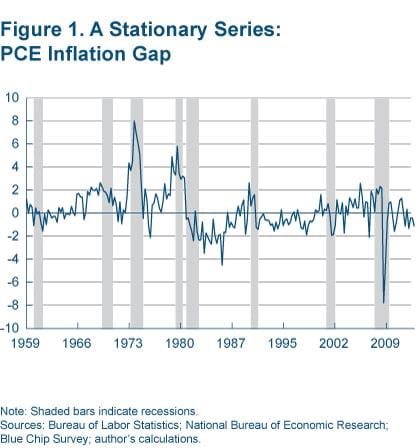
A stationary variable (or process) is one whose basic statistical properties, such as the mean and the variance, remain constant over time. In other words, a stationary variable varies around a fixed level, one that neither grows nor declines. A nonstationary variable, on the other hand, varies around a level that grows or declines over time. Figure 1 plots an example of a series, the PCE inflation gap, that would qualify as stationary. Over time the series fluctuates around a mean of 0.30, and the dispersion of the fluctuations on average is constant.

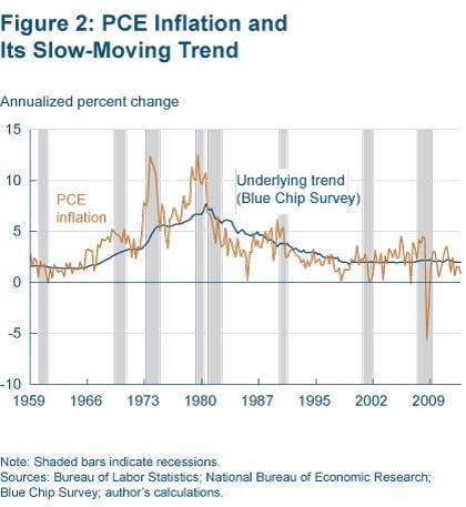
In contrast, figure 2 shows a nonstationary series, quarterly annualized PCE inflation. Clearly there seems to be a slow-moving trend component, which rises in the 1970s (a period dubbed the Great Inflation) and then continues to fall over the subsequent decades.

Forecasting methodologies that do not account for this slow-moving trend are naturally going to fare poorly in forecasting PCE inflation, especially two years out and longer. By construction, models that assume a stationary specification for inflation generate long-term forecasts that converge to the sample mean. For example, if our estimation sample spans 1959 to 2012, the inflation forecast three to four years out (beginning 2013:Q1) would be something around 3.5 percent (which is the average PCE inflation rate from 1959 to 2012). Given that long-term inflation expectations from various surveys are well-anchored around the Federal Reserve’s long-term inflation objective of 2 percent, this is clearly an unreasonable forecast, and it results from failing to account for the slow-moving trend.

If the estimation sample begins instead in 1985, the model’s long-term forecast would be more reasonable—somewhere around 2 percent, since the inflation mean in this sample is close to 2 percent. Though estimating a model with only post-1985 data may be reasonable in the case of a univariate model (in which inflation is the only variable being modeled and of interest), it is not in the case of multivariate models. In multivariate models, the forecasts of other variables, like real GDP, are also of interest, and to capture rich historical multivariate dynamics, one needs to go as far back as possible.

Inflation Forecasting Using the Trend

Fortunately, some researchers (Kozicki and Tinsley (2001), Clark and McCracken (2008), Clark (2011), and Faust and Wright (2012), to name a few) have devised a clever approach to capture this slow-moving inflation trend. It involves using expectations for inflation in six to ten years from the Blue Chip Survey or the forecasts of inflation over the next 10 years from the Survey of Professional Forecasters (SPF).¹² The surveys ask respondents for their predictions of inflation, and these predictions are used to estimate the underlying inflation trend. The history of responses goes back to 1979 for the Blue Chip survey and 1991 for the SPF.

Figure 2 plots the inflation trend that is calculated with Blue Chip expectations (which we use here due to the survey’s longer history).³ Comparing this estimated trend to PCE inflation suggests that the estimated trend easily passes as a reasonable measure of the underlying slow-moving trend level of inflation.

The estimated trend is used to produce a forecast for inflation in the following way. First we define an “inflation gap” as the deviation of PCE inflation from the estimated trend.⁴ Figure 1 plots this constructed inflation-gap series. A quick visual inspection leads one to conclude that the series is fairly stationary. Given this fact, we can model it with a stationary specification.

Finally, the forecasts coming out of this specification would be of the PCE inflation gap, so to obtain the implied PCE inflation forecasts, we would add back in the trend level of inflation (its most recent value).⁵

I illustrate this technique on two types of commonly used, simple statistical time series models: a univariate (single-equation) and multivariate (multi-equation) setting. To test whether incorporating the underlying trend improves the inflation forecast, we estimate two specifications for each type of model. One uses PCE inflation—the benchmark specification—and one uses the PCE inflation gap. Then we compare the accuracy of forecasts for the future rate of PCE inflation.⁶ Our forecast evaluation period spans 1990:Q1 to 2013:Q1.

Specifications estimated with the inflation gap generate superior forecasts throughout the forecast horizon, with the greatest gains achieved in the medium and long term (two to three years out). The gains in forecast accuracy are of substantial magnitude, ranging from 10 percent in the short term to about 30 percent in the long term. Furthermore, in the multivariate setting, the forecast accuracy of variables other than inflation is statistically unaffected, which is a big benefit. It means that existing statistical models can quickly and easily be adjusted to incorporate the inflation-gap approach, improving inflation forecasts without sacrificing the accuracy of other variables.

The Forecast Exercises

I conduct the forecast exercises with univariate and multivariate models because both are in common use. Though simple, univariate models are useful for inflation forecasting as they have been shown to be very hard to beat (see Atkenson and Ohanian (2001) and Stock and Watson (2009)), and therefore they are often used as a benchmark against which other sophisticated models are evaluated.

Univariate models use current and past values of inflation to forecast future inflation, and because inflation is a fairly persistent process, this approach can be helpful. However, in other cases, multivariate models are required. One obvious example is monetary policy. Policymakers must know about the potential impact of changes in one variable on others, so they require systemically consistent forecasts of multiple variables.

Univariate Setting

The univariate model uses information only from past values of PCE inflation.

To construct the benchmark case, I estimate a quarterly regression model that forecasts inflation using the past four values of the quarterly annualized percent change in PCE inflation. The regression analysis determines the weights that should be assigned to the past four quarterly values of PCE inflation in forecasting the next period’s inflation. I estimate this regression model in a recursive fashion beginning with a sample from 1959:Q1 to 1989:Q4 (124 quarters). Then, using the estimated parameters, I generate forecasts one quarter to 12 quarters out (for example, 1990:Q1 to 1992:Q4) and then compute the forecast errors for each of the 12 forecast horizons. Then I add another quarterly data point to the sample, re-estimate, and again compute the forecast accuracy and so on until I reach the end of the estimation sample, 2010:Q1.

This way, the forecast made at 2010:Q1 would extend all way to 2013:Q1 (12 quarters out), the latest quarter for which we had PCE inflation data. So our forecast evaluation period spans 1990:Q1 to 2013:Q1. Doing this exercise gives us 82 forecast errors for each of the 12 forecast horizons. I square each of the forecast errors, and then for each forecast horizon take the mean of these squared errors to obtain the corresponding mean squared error (MSE).

To construct the inflation-gap case, I repeat this same exercise but this time I estimate the quarterly regression model with the PCE inflation gap. At each recursive run, the model spits out the forecast of the PCE inflation gap, to which I add the value of the slow-moving trend that would be available at that point in time, generating the corresponding implied PCE inflation forecast. I then compute the relative MSE for each of the horizons by dividing the MSEs from the inflation-gap specification by the MSEs of the benchmark.

Figure 3 plots these relative MSEs. All relative MSEs are below one, implying that the inflation-gap model produces more accurate forecasts. Importantly, the relative MSE decreases linearly, meaning that the degree of accuracy increases as the forecast horizon lengthens. For example, the relative MSEs one and 12 quarters out are 0.93 and 0.69, respectively, indicating that the forecasts coming out of the inflation-gap model are about 7 percent more accurate than the benchmark one quarter out and 31 percent more accurate 12 quarters out.

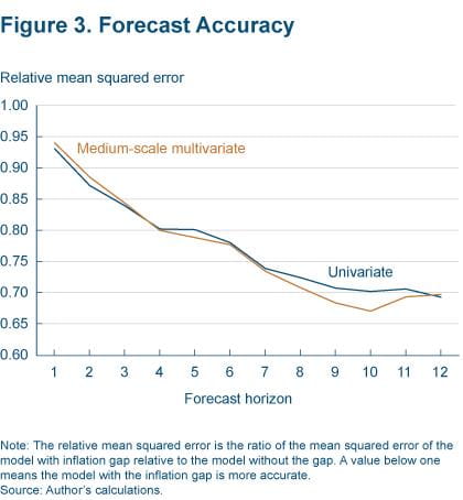
Figure 4 plots the five-quarter moving average of the squared forecast errors corresponding to the 12-quarter-out forecast horizon from both model specifications.⁷ Clearly, the model that uses the inflation gap generally outperforms the benchmark, and the magnitude of the errors is substantially smaller than in the benchmark.

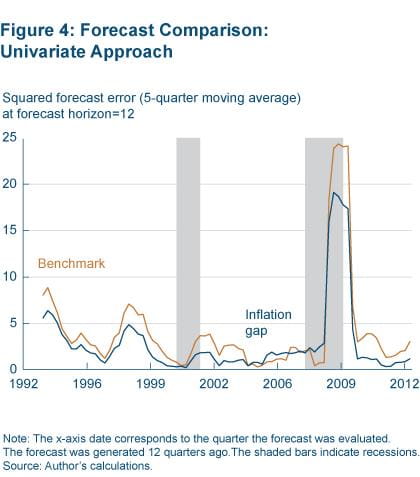
Both models performed relatively poorly at the height of the financial crisis, as evidenced by a spike around the end of 2008. For example, in 2008:Q4 and 2009:Q1 the overall annualized quarterly PCE inflation rate declined 5.6 percent and 2.2 percent, respectively. Not surprisingly, the 12- quarter-ahead inflation forecast (the forecast for 2008:Q4) from the benchmark model made at the end of 2005 was 3.9 percent (about the same as the sample mean for 1959-2005), whereas from the inflation-gap model it was 2.5 percent (a little above the underlying trend level as of 2005:Q4). The squared forecast errors from the two models were 88 points and 65 points, respectively, in 2008:Q4 (not obvious in the figure since it reports the five-quarter moving average).

Multivariate Setting

One class of multivariate model often used for forecasting and policy analysis is Bayesian vector autoregressions (BVARs). A BVAR is primarily a multiple time series generalization of the (autoregressive) model used in our earlier univariate case.

Accordingly, I employ a BVAR model described in Beauchemin (2011). This model contains ten variables—real GDP, core PCE price index, PCE price index, total nonfarm payroll employment, nonfarm business productivity, nonfarm business compensation, the West Texas intermediate crude oil price (WTI), the Commodity Research Bureau (CRB) index of raw industrial commodity prices (non-energy and non-food), the CRB price index for foodstuffs, and the federal funds rate.⁸

To construct the benchmark case, I perform a recursive exercise similar to that of the univariate case. Specifically, I begin the estimation using a sample from 1959:Q1 to 1989:Q4. Then I forecast up to 12 quarters out, compute the associated forecast errors, and proceed by adding another quarterly data point and re-estimating and so on until I reach 2010:Q1. Then for each forecast horizon, I square each of the computed forecast errors (again, 82 errors) and compute the corresponding MSEs.

To compute the inflation-gap multivariate case, I repeat this same exercise, but replace the PCE price index and the core PCE price index with the PCE inflation gap and a similarly constructed core-PCE-inflation gap. Finally, just like in the univariate setting, I compute the relative MSEs for each of the horizons (by dividing the MSEs from the inflation-gap specification by the MSEs from the benchmark case).

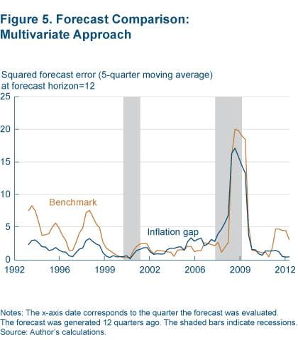
Figure 3 plots the relative MSEs for each of the 12 forecast horizons. They are all below one, implying that the model estimated with the PCE inflation gap is significantly more accurate in forecasting inflation than the benchmark, with the greatest gains in accuracy achieved at forecast horizons of one year and beyond. For example, the improvement in accuracy at one, two, and three years out is 20 percent, 29 percent, and 30 percent, respectively.

Figure 5 plots the five-quarter moving average of the squared forecast errors corresponding to the 12-quarter-out forecast horizon from both the benchmark and the inflation-gap specifications. Consistent with the univariate case, the multivariate model that uses the inflation gap generally outperforms the benchmark, as judged by its lower squared forecast errors. Furthermore, the relative forecast performance of the other variables of the BVAR is not statistically affected. If anything, it is slightly better.⁹

Conclusion

We have seen that to accurately forecast the future rate of inflation, it is imperative to account for the slow-moving, underlying trend in inflation. This is more so the case for medium to long-run forecasts for inflation. Importantly, this forecast horizon coincides with the FOMC’s inflation-monitoring horizon. Language in FOMC meeting statements explicitly ties guidance about the future path of the federal funds rate to inflation forecasts one to two years out, as well as to progress in reducing the unemployment rate.

Incorporating the underlying inflation trend into standard statistical time series models using the technique laid out in this Commentary is simple and easy. Doing so may lead to increased accuracy of inflation forecasts, and in turn a more informed expectation of the future federal funds rate.