

- Share
Postpandemic Nominal Wage Growth: Inflation Pass-Through or Labor Market Imbalance?
Measures of wage growth have increased substantially during and after the pandemic compared to their average levels in the decade before. Does higher wage growth reflect compensation for a higher cost of living, brought about by an increase in inflation in the past two years? Or has an imbalance between strong labor demand and restrained labor supply lifted wage growth? Using a new empirical wage Phillips curve model, we find that the increase in wage growth largely reflects the pass-through of higher inflation and does not reflect labor market imbalances. The model forecasts a decline in wage growth to about 3 percent annually by 2025.

The views authors express in Economic Commentary are theirs and not necessarily those of the Federal Reserve Bank of Cleveland or the Board of Governors of the Federal Reserve System. The series editor is Tasia Hane. This paper and its data are subject to revision; please visit clevelandfed.org for updates.
The sharp economic contraction caused by the COVID-19 pandemic was followed by a rapid recovery and sustained expansion of labor market activity. Job openings rose to record levels, and employers noted widespread labor shortages, both of which indicated that the demand for labor had outpaced the supply.1 Meanwhile, inflation rose to its highest level since the 1980s. Throughout the postpandemic period, various measures of nominal wages have also accelerated, thus raising the question of whether higher wage growth reflects the pass-through of inflation or the imbalance between demand and supply in the labor market.
Analysts often interpret the cyclical behavior of wage growth by means of a wage Phillips curve that relates wage growth to its past values, past inflation rates, or both and to the unemployment rate.2 However, the unemployment rate may not adequately capture wage pressures arising from large imbalances between demand and supply in the labor market. Indeed, the average unemployment rate from 2021:Q2 to 2023:Q1 was the same as during the prepandemic economic expansion from 2016:Q1 to 2019:Q4 (4.2 percent), even as the average rate of job openings had increased sharply and the labor force participation rate had fallen substantially.
In this Economic Commentary, we investigate the source of the recent increase in wage growth by using a new empirical wage Phillips curve. Instead of responding to fluctuations in the unemployment rate, wage growth in our empirical model adjusts to restore imbalances between the long-run levels of macroeconomic variables. The relevant variables are selected based on structural models of the business cycle that incorporate a sluggish adjustment of wages in response to economic conditions. In the canonical structural model, wage growth varies in order to restore the long-run relationship between real wages and the marginal value of time (Erceg, Henderson, and Levin, 2000). A high consumption level or long hours worked raises people’s marginal value of time so that a higher real wage is required to entice them to take on more work. Accordingly, our empirical wage Phillips curve includes, as a key driver of wage growth, the estimated deviations from the long-run relationship among the wage level, the price level, real consumption, and hours. That relationship can be interpreted as a long-run labor market equilibrium in line with the structural models of wage growth.
Our empirical wage Phillips curve, estimated on a sample of prepandemic time series, predicts the postpandemic increase in wage growth well. We use the estimated model to examine the role of inflation by comparing a forecast of wage growth conditional on the actual path of inflation with a forecast conditional on a counterfactual, constant inflation rate of 1.5 percent annually, its average level in the decade before the pandemic. The counterfactual exercise indicates that the elevated inflation rate over the past two years accounts for much (four-fifths) of the increase in wage growth. During that time, the estimated deviation of the long-run labor market equilibrium displayed a sharp decline and recovery, dynamics that point to substantial downward and upward pressures of labor market imbalances on wage growth. However, the contribution of labor market imbalances to the average level of wage growth did not increase from their contribution before the pandemic. Thus, we conclude that the post-pandemic increase in wage growth largely reflects higher inflation and does not reflect labor market imbalances.3
While wage growth remains higher than before the pandemic, inflation has come down from its recent peak, and wage pressure as measured by the model’s estimated deviation of the long-run labor market equilibrium has already begun to ease. Both these developments point to declines in future wage growth. Indeed, the estimated model’s forecast of wage growth declines gradually to about 3 percent annually by 2025.
An Empirical Wage Phillips Curve Model
Several different wage indices are available to track the overall wage level in the economy. Although they generally show increases in wage growth since the pandemic, their short-run dynamics can differ noticeably as some of the measures display greater volatility or persistence than others. For our analysis, we focus on the employment cost index (ECI) for civilian workers. The ECI is a comprehensive measure that includes wages, salaries, and benefits and is designed to mitigate bias arising from changes over time in the composition of employment across industries and occupations. For example, if a recession leads to the destruction of low-wage service jobs while maintaining all other jobs, the ECI would be unaffected.
Our econometric model is a vector error correction model (VECM) with four variables: wage growth, inflation, real consumption growth, and hours growth.4 The model consists of four equations, with each describing one of the variables as the sum of three terms.5 The first term is the “error correction term,” so called because it adjusts each variable to correct temporary deviations from the joint long-run, “cointegrating” relationship between the levels of wages, prices, real consumption, and hours. The second term consists of lags of all four variables to describe the short-run dynamics of each variable. The third term is a random disturbance that captures unpredictable variation. An advantage of cointegration in time series models is that it can help improve forecasts by exploiting the stochastic trends shared by variables in the model. The equation for wage growth is our empirical wage Phillips curve, and the equations for inflation, real consumption growth, and hours growth are auxiliary equations.6
We choose a sample of quarterly time series from 1982:Q1 to 2019:Q4, thus preventing the pandemic recession from influencing the parameter estimates.7 We estimate the model parameters using maximum likelihood estimation.
Forecast Accuracy
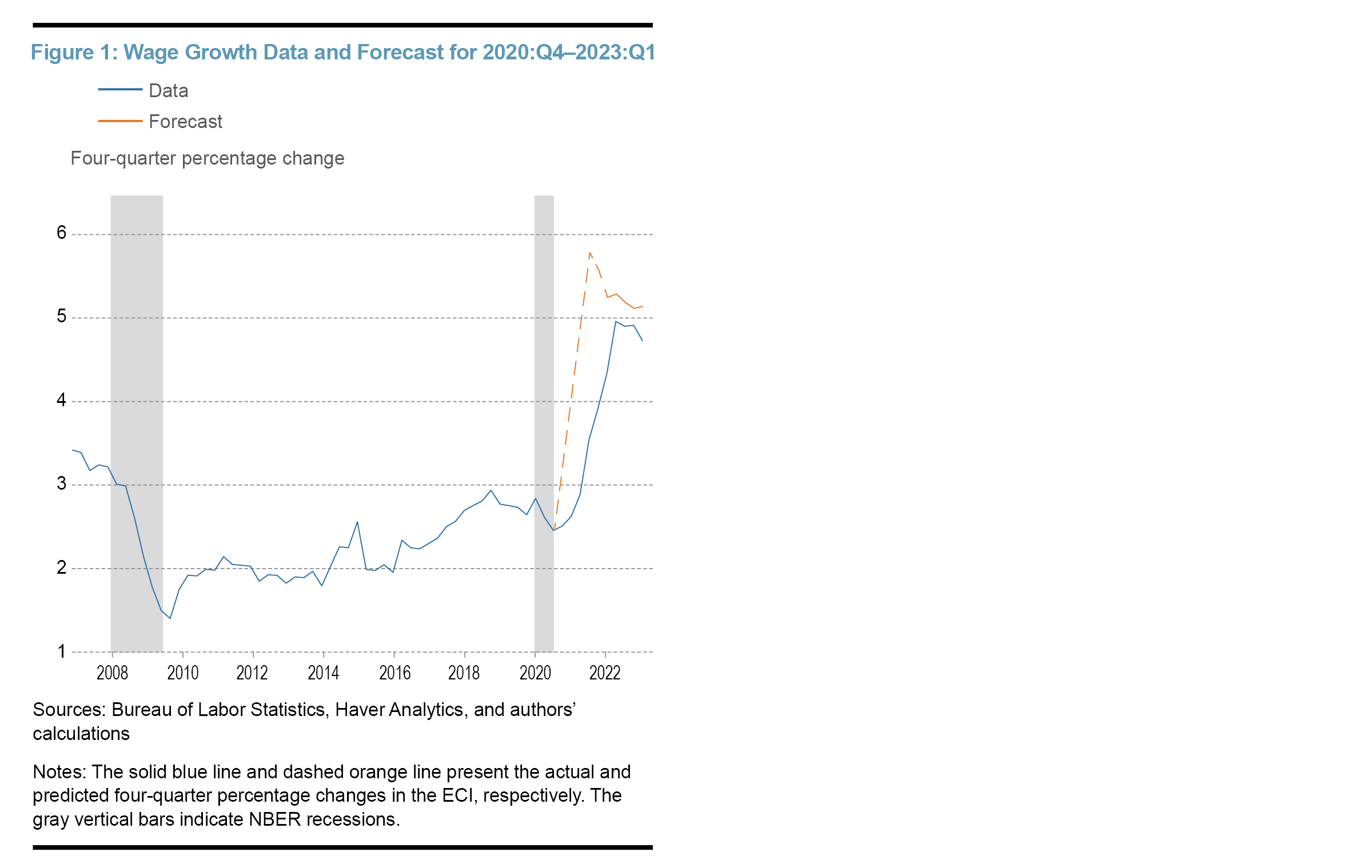
Average wage growth increased 2.1 percentage points from 2.2 percent during the labor market expansion from 2010:Q1 to 2019:Q4 to 4.3 percent during the recent period from 2020:Q4 to 2023:Q1.8 Is the estimated wage Phillips curve model a useful tool for assessing the roles of inflation pass-through and labor market imbalances in the increase? A minimum requirement is that the estimated model predicts the recent evolution of wage growth fairly accurately. If the model cannot explain what happened, it cannot explain why it happened.
We assess the model by comparing its out-of-sample forecast of recent wage growth with the data. Figure 1 plots year-over-year wage growth and the model forecast from 2020:Q4 to 2023:Q1. To produce the forecast, we initialize the estimated model with data observations until 2020:Q3, a period that includes the initial quarter of the recovery from the pandemic recession but excludes the subsequent rise in inflation. The model equations are then combined to predict each variable in 2020:Q4 and onward. The estimated model predicts the path of wage growth fairly successfully: The forecast of wage growth tracks the data as they increase rapidly to a level above 5 percent. While the forecast jumps immediately after the initial recovery in real consumption and hours, the increase in actual wage growth built up over a few quarters.
Inflation Pass-Through
Having established that the model’s out-of-sample forecast captures the recent increase in wage growth, we now use the wage Phillips curve to gauge the role of pass-through from inflation to wages.
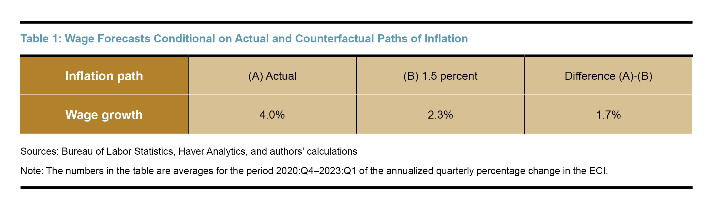
We isolate the pass-through from inflation from late 2020 through early 2023 by conducting a counterfactual exercise. Specifically, we use the estimated wage Phillips curve to generate two conditional forecasts of wage growth that assume different paths for inflation. The first conditional forecast is based on the time series data of the price level, real consumption, and hours through 2023:Q1. The second one is a counterfactual forecast conditional on a price level that increases from 2020:Q4 onward at a constant rate of 1.5 percent annually, the average inflation rate during the economic expansion from 2010:Q1 to 2019:Q4.
Comparing the forecast of wage growth conditional on the actual path of the price level to the one based on the counterfactual price level path provides an estimate of the pass-through from inflation to wage growth. Table 1 presents the conditional and counterfactual forecasts of wage growth as averages for the period from 2020:Q4 to 2023:Q1. Based on the actual path of the price level, the conditional forecast of wage growth is 4.0 percent, close to but a little below the average of actual ECI growth during the period. The counterfactual path of the price level produces a weaker conditional wage growth forecast of 2.3 percent. Hence, our estimated wage Phillips curve indicates that the recent increase in inflation accounts for 1.7 percentage points, or four-fifths, of the 2.1 percentage point increase in average wage growth for the period 2020:Q4–2023:Q1 compared to 2010:Q1–2019:Q4. This conclusion is based on the estimated dynamic relationship between wage growth and inflation over the sample period. A caveat is that the pass-through of prices to wages may have changed since the pandemic. For example, if the increase in inflation made workers more attuned to the eroding purchasing power of their wages, wage growth may have become more sensitive to inflation than usual, in which case the pass-through of inflation to wage growth could exceed our estimate. On the contrary, if the rapid, unexpected increase in inflation caught wage-setters by surprise, the pass-through to wage growth could be smaller than our estimate.
As higher inflation accounts for the bulk of the predicted increase in wage growth, our estimated wage Phillips curve leaves limited room for other contributing factors. Nevertheless, it is instructive to take a closer look at the role played by labor market imbalances in the increase in wage growth.
Labor Market Imbalance
A key driving factor of wage growth in the empirical model is the error correction term, which describes what portion of wage growth can be attributed directly to the deviation in the previous quarter from the joint long-run equilibrium relationship among the wage level, the price level, real consumption, and hours worked. These macroeconomic variables were selected based on economic models in which households make labor supply decisions. Such models contain a labor supply curve, on which real wages are proportional to the marginal value of time that depends on consumption and hours worked. In particular, models with sluggish adjustment of wages feature a wage Phillips curve that leads wage growth to respond to deviations from the long-run relationship between real wages and the marginal value of time. This theoretical motivation suggests that the long-run equilibrium relationship between the variables in our model may describe a long-run labor market equilibrium.9 The deviations from the long-run labor market equilibrium then have a natural interpretation as labor market imbalances. Thus, the error correction term provides the contribution of labor market imbalances to wage growth.10
To visualize the influence of labor market imbalances on wage growth, Figure 2 presents the error correction term along with year-over-year wage growth. During each of the economic expansions that preceded the recessions of 1990–1991, 2001, and 2008–2009, the error correction term increased gradually to reach a peak a few quarters before the recession, a fact suggesting that the term is not only a driver but also a predictor of the cyclical dynamics of wage growth.
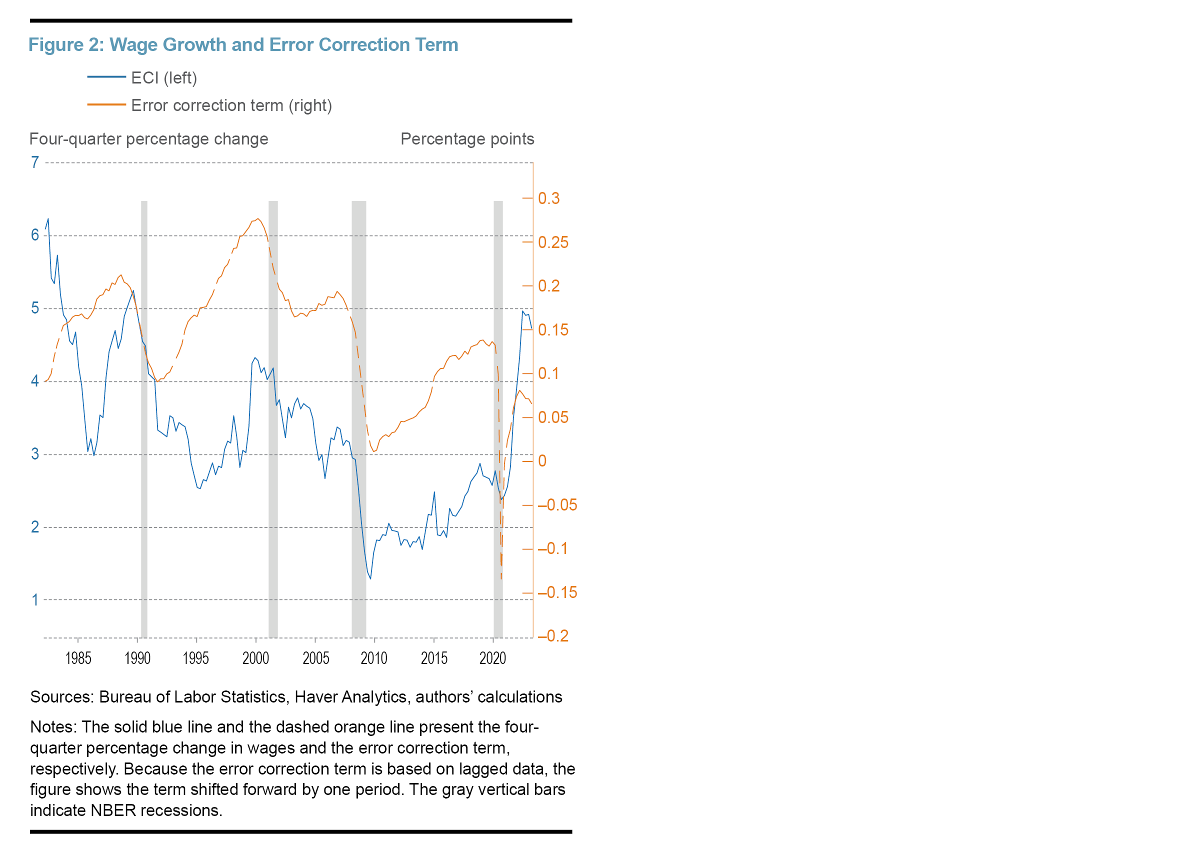
The last few years of observations in Figure 2 shed light on the role of labor market imbalances in the current expansion.11 The error correction term dropped more sharply and rebounded more rapidly than during any of the previous cycles in the sample. The dramatic V-shaped pattern is similar to those followed by real consumption and hours worked, two of the time series used in the estimation. The decline in the error correction term put downward pressure on wage growth, but this pressure soon reversed, turning into upward pressure. In this way, labor market imbalances appear to have been an especially important source of cyclical pressures on wage growth in the postpandemic period.
Despite the large cyclical swings, however, the error correction term does not account for the increase in average wage growth in the postpandemic period compared to average wage growth during the labor market expansion of 2010–2019. The average level of the error correction term in the period since 2020:Q4 lies below its average level during the previous labor market expansion, a situation which rules out the possibility that the contribution of labor market imbalances to average wage growth has increased.12 Taken together, our analysis based on the empirical wage Phillips curve implies that the postpandemic increase in wage growth is largely due to higher inflation and does not reflect labor market imbalances.
Wage Forecast
Looking ahead, wage growth will likely decline in the foreseeable future. Inflation has come down from its peak in mid-2022, pointing to a decline in wage growth from diminishing inflation pass-through. Moreover, the error correction term in Figure 2 has moderated since early 2022, suggesting that the recent upward pressure from labor market imbalances on wage growth is also diminishing. Figure 3 provides a medium-term forecast of wage growth based on the estimated model initialized with data until 2023:Q1. Year-over-year wage growth is projected to decline to 3.3 percent by 2024:Q4 and edge down further to 2.8 percent by 2025:Q4 simultaneous with the projected declines in the year-over-year inflation rate to 2.6 percent by 2024:Q4 and 2.2 percent by 2025:Q4. Evidently, the model interprets a level of wage growth around 3 percent as consistent with 2 percent inflation, in accordance with the view of policymakers (Board of Governors of the Federal Reserve System, 2023). Of course, this forecast is uncertain, and actual outcomes may differ as a result of unforeseen shocks.
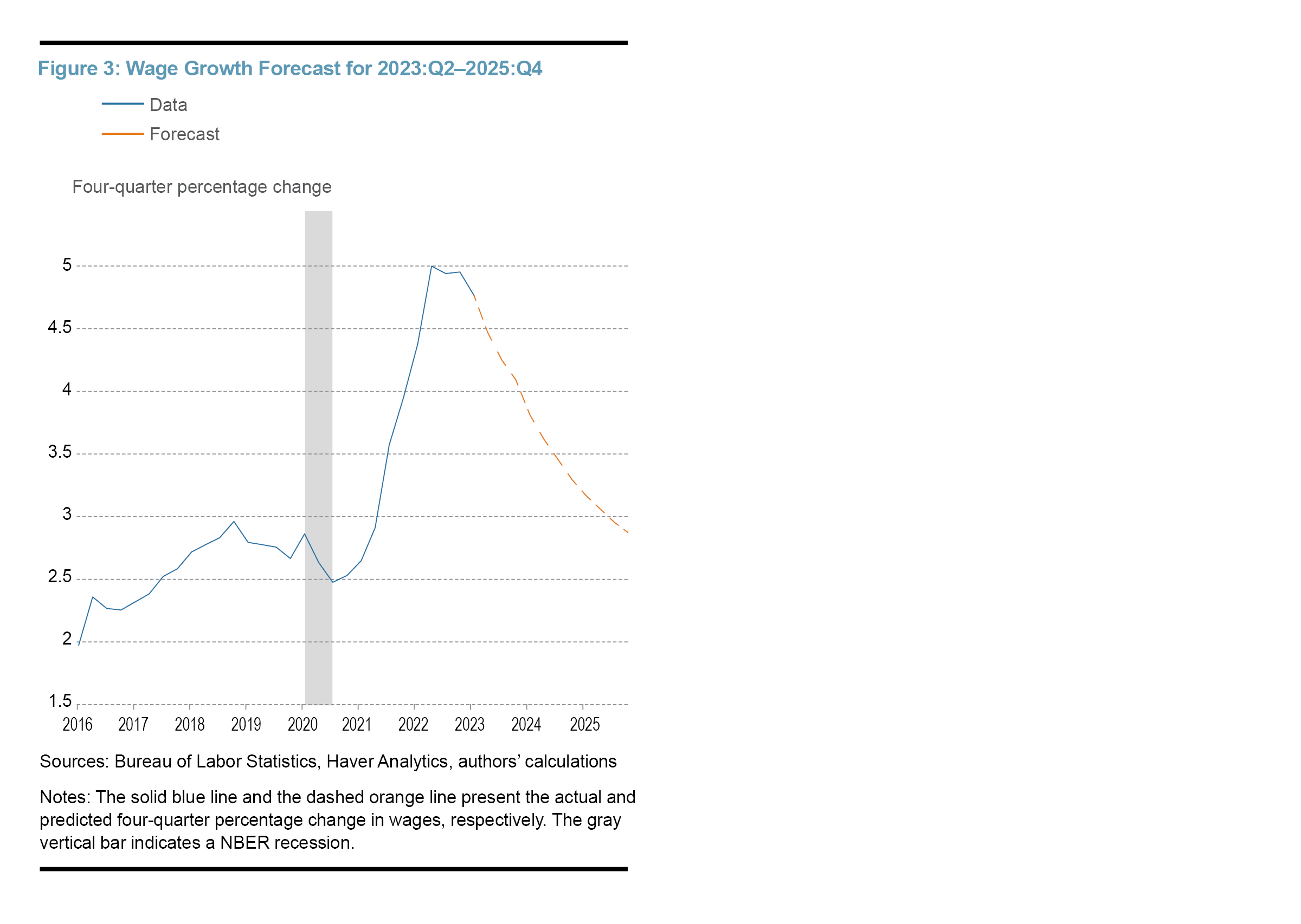
The forecast of the estimated model calls for further declines in wage growth and inflation; the model also implies that wage growth would remain elevated if inflation remained persistently high. We gauge the importance of the forecasted decline in inflation for the forecasted decline in wage growth by conducting another counterfactual exercise. This exercise assumes that inflation remains fixed during the forecast horizon at 4.1 percent, the annualized rate in 2023:Q1, and employs the estimated wage Phillips curve and the auxiliary equations for real consumption growth and hours growth to generate a conditional forecast of wage growth. Under the counterfactual path of persistently high inflation, year-over-year wage growth barely declines, edging down from 4.7 percent in 2023:Q1 to 4.6 percent in 2025:Q4. Like the recent rise in wage growth, its expected decline appears to largely reflect inflation pass-through.
Conclusion
The pandemic-induced recession and the rapid subsequent recovery of the US economy gave rise to higher inflation and labor market imbalances. To estimate the role of these factors in explaining the postpandemic increase in wage growth, we have estimated an empirical wage Phillips curve in the form of a VECM that captures the influence on wage growth of the deviations between key macroeconomic variables from their long-run equilibrium relationship, a measure of labor market imbalances. Our empirical wage Phillips curve successfully predicts the recent increase in wage growth and indicates that it is largely due to the pass-through of higher inflation since the pandemic. While labor market imbalances have been large in the postpandemic period, they induced both downward and upward pressures on wage growth and do not account for the increase in average wage growth. A forecast of the estimated model has wage growth decline gradually over the medium term.
References
- Blanchflower, David G., Alex Bryson, and Jackson Spurling. 2022. “The Wage Curve After the Great Recession.” Working paper 30322. National Bureau of Economic Research (August). https://www.nber.org/papers/w30322.
- Board of Governors of the Federal Reserve System. 2023. “Transcript of Chair Powell’s Press Conference, May 3, 2023.” https://www.federalreserve.gov/monetarypolicy/fomcpresconf20230503.htm.
- Erceg, Christopher J., Dale W. Henderson, and Andrew T. Levin. 2000. “Optimal Monetary Policy with Staggered Wage and Price Contracts.” Journal of Monetary Economics 46 (2): 281–313. https://doi.org/10.1016/s0304-3932(00)00028-3.
- Galí, Jordi, and Luca Gambetti. 2020. “Has the U.S. Wage Phillips Curve Flattened? A Semi-Structural Exploration.” In Changing Inflation Dynamics, Evolving Monetary Policy, edited by Gonzalo Castex, Jordi Galí, and Diego Saravia, 149–72. Series on Central Banking, Analysis, and Economic Policies, no. 27. Santiago, Chile: Central Bank of Chile. https://repositoriodigital.bcentral.cl/xmlui/handle/20.500.12580/4877.
- Glick, Reuven, Sylvain Leduc, and Mollie Pepper. 2022. “Will Workers Demand Cost-of-Living Adjustments?” FRBSF Economic Letter, no. 2022-21 (August). https://www.frbsf.org/economic-research/publications/economic-letter/2022/august/will-workers-demand-cost-of-living-adjustments/.
- Hajdini, Ina, Edward S. Knotek II, John Leer, Mathieu O. Pedemonte, Robert W. Rich, and Raphael S. Schoenle. 2023. “Low Passthrough from Inflation Expectations to Income Growth Expectations: Why People Dislike Inflation.” Working Paper 22-21R, Federal Reserve Bank of Cleveland (March). https://doi.org/10.26509/frbc-wp-202221r
- Jordà, Òscar, and Fernanda Nechio. 2022. “Inflation and Wage Growth Since the Pandemic.” Working paper 2022-17. Federal Reserve Bank of San Francisco (April). https://doi.org/10.24148/wp2022-17.
- Kivedal, Bjørnar Karlsen. 2018. “A New Keynesian Framework and Wage and Price Dynamics in the USA.” Empirical Economics 55 (November): 1271–1289. https://doi.org/10.1007/s00181-017-1320-8.
- Knotek II, Edward S., and Saeed Zaman. 2014. “On the Relationships between Wages, Prices, and Economic Activity.” Economic Commentary, no. 2014-14 (August). https://doi.org/10.26509/frbc-ec-201414.
- Powell, Jerome H. 2022. “Inflation and the Labor Market.” Remarks by Jerome H. Powell, Chair, Board of Governors of the Federal Reserve System, November 30, 2022. Washington DC: Hutchins Center on Fiscal and Monetary Policy, Brookings Institution. https://www.federalreserve.gov/newsevents/speech/powell20221130a.htm.
- Smith, Christopher L. 2014. “The Effect of Labor Slack on Wages: Evidence from State-Level Relationships.” FEDS Notes. Board of Governors of the Federal Reserve System (June). https://doi.org/10.17016/2380-7172.0021.
Endnotes
- Powell (2022) observed that “In the labor market, demand for workers far exceeds the supply of available workers, and nominal wages have been growing at a pace well above what would be consistent with 2 percent inflation over time.” Return to 1
- For examples, see Knotek and Zaman (2014), Smith (2014), Galí and Gambetti (2020), and Glick et al. (2022). Return to 2
- Our model abstracts from expectations about future inflation or wages. Other research examines the role of expected inflation on wage growth. Glick et al. (2022) find a substantial influence of inflation expectations, and Jordà and Nechio (2022) report that the influence has increased since the pandemic. While this research finds a substantial effect on actual wage growth, Hajdini and others (2023) examine a 2022 survey of consumers and report a relatively modest effect of expected inflation on expected wage growth. Return to 3
- Kivedal (2018) also uses a VECM to estimate a wage Phillips curve, but his model contains the unemployment rate rather than real consumption or hours because the model is based on a sticky price model with unemployment. Return to 4
- Algebraically, the VECM can be written as ∆yt = A(B’yt-1+α0)+α1∆yt-1+…+ αp-1∆yt-p+1+ εt, where the vector yt contains the wage level, the price level, real consumption, and hours worked in quarter t, A, B, α0, α1, …, αp-1 are coefficient matrices, and εt is a vector of innovations. The term A(B’yt-1+α0) is the error correction term. Return to 5
- The data for the price level, real consumption, and hours are, respectively, the personal consumption expenditures (PCE) price index, real PCE on nondurable goods and services constructed as a Fisher index using the series of real PCE and real PCE on durable goods according to the “chain-subtraction” method, and the hours of all persons in the business sector. Return to 6
- Each time series is expressed in logarithms, and each variable is calculated as the change in the respective time series. For example, the wage growth rate is obtained as the change from the previous quarter in the logarithm of the wage level. The VECM requires that the level of each time series has a unit root, so its change is stationary. In the sample, unit root and stationarity tests indicate that the wage level, the price level, real consumption, and hours contain a unit root, while their changes are stationary. There is one cointegrating relationship among the wage level, the price level, real consumption, and hours, according to the Johansen trace and maximum eigenvalue tests. The number of lags of each variable of the model is set at its largest value recommended by the Schwarz and Hannan Quinn information criteria and is equal to 3 (= p-1). Return to 7
- Wage measures other than the ECI also accelerated. Growth in compensation per hour in the business sector, average hourly earnings growth, and the Atlanta Fed wage growth tracker increased, respectively, by 1.8 percentage points, 2.2 percentage points, and 2.2 percentage points. Return to 8
- Although the theory imposes restrictions on the signs and magnitudes of coefficients in the long-run labor market equilibrium, we do not impose such restrictions in the estimated model to enhance its forecasting performance. Return to 9
- Our modeling approach circumvents the challenge of measuring labor market imbalances directly in the labor market data. Evidence of a restrained labor supply could be seen, for example, in weak labor force data, while strong labor demand could be manifested in high levels of job openings and indicators of job-to-job transitions such as quits. The challenge with such an alternative approach is twofold. First, the best way of combining multivariate labor market data into a single measure of labor market imbalances may not be obvious. Second, some available data may not adequately capture the intended concept. For example, Blanchflower and others (2022) discuss a number of drawbacks of job openings data, one of which is that posting a job vacancy has become increasingly easy and cheap and thus the number of job openings may not provide an accurate reading of labor market tightness. Return to 10
- The out-of-sample error correction term is calculated by multiplying the estimate of the long-run coefficient matrix of the VECM with the out-of-sample data matrix. Return to 11
- The average of the error correction term was 0.056 in the period 2020:Q4–2023:Q1, below the average of 0.082 for the period 2010:Q1–2019:Q4. As the figure shows, the contribution of the error correction term to the average level of wage growth during economic expansions has declined in each of the expansions since the 2001 recession. Return to 12
Suggested Citation
DeLuca, Martin, and Willem Van Zandweghe. 2023. “Postpandemic Nominal Wage Growth: Inflation Pass-Through or Labor Market Imbalance?” Federal Reserve Bank of Cleveland, Economic Commentary 2023-13. https://doi.org/10.26509/frbc-ec-202313
This work by Federal Reserve Bank of Cleveland is licensed under Creative Commons Attribution-NonCommercial 4.0 International

