

- Share
Has the Real-Time Reliability of Monthly Indicators Changed over Time?
Economic data are routinely revised after they are initially released. I examine the extent to which the real-time reliability of six monthly macroeconomic indicators important to policymakers has remained stable over time by studying the time-series properties of their short-term and long-term revisions. I show that the revisions to many monthly economic indicators display systematic behaviors that policymakers could build into their real-time assessments. I also find that some indicators’ revision series have varied substantially over time, suggesting that these indicators may now be less useful in real time than they once were. Lastly, I find that substantial revisions tend to occur indefinitely after the initial data release, a result which suggests a certain degree of caution is in order when using even thrice-revised monthly data in policymaking.
The views authors express in Economic Commentary are theirs and not necessarily those of the Federal Reserve Bank of Cleveland or the Board of Governors of the Federal Reserve System. The series editor is Tasia Hane. This paper and its data are subject to revision; please visit clevelandfed.org for updates.
Economic policymakers carefully assess all recent economic data for clues about the current state of the economy and where it may be headed. However, a unique feature of economic data is that they are subject to revisions. Knowing that this is the case, policymakers aim to strike a balance in their use of the incoming data, taking some signals from the data while not over interpreting them, aware that the real-time data provide an imperfect measure of economic activity.
In this article I examine the stability over time of the reliability of real-time monthly data. At an intuitive level, I define “reliability” as the similarity of the real-time values to their subsequent revised values. To be more precise, I will assess the reliability of the real-time data in terms of the statistical properties of the revisions.1 The smaller and less statistically biased are the revisions to a given data series, the more reliable I consider the real-time data for that series to be.
This article focuses on monthly indicators for two reasons. First, as relatively high-frequency indicators of economic activity, monthly indicators are often the main new source of information in policy decisions. Second, relative to quarterly indicators, monthly indicators tend to be more volatile from one observation to the next, which naturally raises questions about their reliability. Hence, an assessment of the information content and revision properties of monthly indicators is particularly important for their best use in economic decision making.
I will show that the revisions to many monthly economic indicators display systematic behaviors that policymakers could build into their real-time assessments and that some of these behaviors have changed over time.
Revisions
For many data series, the values initially reported are changed months after the initial value is published and often more than once. The difference between the measured values at two different times is called a revision. For each series that I consider, I analyze two different types of revisions that I call “short-term” revisions and “long-term” revisions.
Short-term revisions result from statistical agencies’ updating preliminary estimates as additional source information becomes available. Each series examined in this article has (at least) a first, second, and third release, with the releases occurring at one-month intervals.2 Taking the data on payroll employment as an example, the Bureau of Labor Statistics (BLS) publishes the “first preliminary” estimate based on less than the total sample and the “final revised sample-based estimate” two months later when nearly all the reports in the sample have been received.3 I call the revision from the first release to the third release the short-term revision. The idea behind this notion of a revision is that it summarizes the maximum amount of new information policymakers obtain about a particular data point of a series within a quarter, and, for some series, before a similar but more encompassing quarterly series becomes available.
Beyond short-term revisions, the value of the indicator reported in a past release can be revised much later. Such revisions are typically the result of either improvements or other changes to the reporting agency’s statistical practices or revisions of seasonal-factor estimates. These processes can continue indefinitely, and so I consider the “long-term” revision to be the revision from the third release up to the present value. Taking the data on industrial production (IP) as an example, the 2002 annual revisions included the application of methods such as chain-weighting and the removal of systematic weather effects from electric power data—methods which previously had been used only for relatively recent data—to the data back to 1972.4 These changes to statistical practices thus caused revisions to data points that were up to 30 years old. To take an example of a more systematic occurrence, seasonal-factor estimates are re-estimated annually. Since every data point in the seasonally adjusted series incorporates a transformation of the raw data using the seasonal adjustment factors, any change to the seasonal adjustment factors will potentially change every data point in the variable’s history.5
Data
I focus on revisions to six monthly economic indicators that are of interest to economic observers and policymakers. Table 1 lists the indicators, the type of measurement taken for each, and the units in which the values are analyzed. Importantly for my purposes, vintages of real-time data are available for each indicator from the Federal Reserve Bank of Philadelphia’s Real-Time Data Research Center.6
| Indicator | Measurement | Units |
|---|---|---|
| Industrial production: Total | Month-over-month growth | Annualized rate, percentage points |
| Industrial Production: Manufacturing | Month-over-month growth | Annualized rate, percentage points |
| Real personal consumption expenditures | Month-over-month growth | Annualized rate, percentage points |
| Housing starts | Housing units | Thousands, seasonally adjusted |
| Nonfarm payroll employment | Monthly change in level | Thousands, seasonally adjusted |
| Index of aggregate weekly hours: Total | Month-over-month growth | Annualized rate, percentage points |
Estimating Reliability over Time
Although users of the real-time economic data hope revisions will be small and idiosyncratic, it is known that revisions can be large and exhibit systematic patterns. For example, it is known in the literature that the growth rate of IP has been systematically understated in real time.
To uncover patterns in the revisions that may have changed over time, I fit to the time-series of revisions a statistical model that allows for both a time-varying mean and time-varying volatility, which are each jointly inferred from the revision data. The mean of a revision series tells us whether or not the underlying data series is systematically revised in a particular direction. For example, if the mean revision is positive, then the initial estimates of the indicator tend to underestimate the value reported in the future. The model’s allowance for a time-varying mean lets it discern if the systematic direction of revisions has changed over time. The volatility of the revisions, on the other hand, measures the size of the typical fluctuation in revisions around the mean. The fact that the model allows for time-varying volatility means that it can determine if the typical size of the fluctuations has changed over time. All else being equal, an indicator with more variable revisions is less reliable in real time.
The statistical model I use is a univariate version of a model explored in Bognanni (2018). I estimate separate univariate versions of the model for both short-term and long-term revisions for each of the six indicators given in table 1. The version of the model estimated for this article focuses on relatively slowly evolving time variation in the means and volatilities of revisions. In doing so, the idea is to restrict attention to changes to the revision process that remain stable enough from one period to the next for policymakers to feel like today’s regularities will not be entirely irrelevant by tomorrow.
Results: Short-Term Revisions
Figure 1 shows, for each economic indicator, the time series of short-term revisions and the estimated time-varying mean of the short-term revisions. The availability of the time series for real-time data begins at different dates for different indicators and hence the region in which the data are not available is shaded in each plot. Note that the time-varying mean is estimated from a model, and any estimation carries some degree of uncertainty about the results. In each plot, the bands around the time-varying mean summarize the estimation uncertainty by highlighting a region of values that has a 68 percent chance of containing the true mean.7
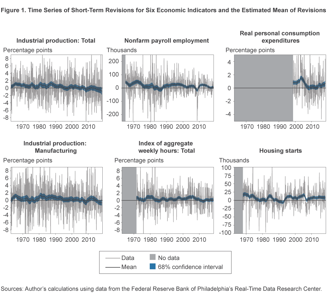
Before turning to indicator-specific estimation results, it is worth taking stock of a few broad regularities that hold across the short-term revision series of all six indicators.
First, the variation in the time-varying means is relatively subtle compared to the overall variability of the revisions. This means that while the mean revision may differ systematically from zero, the difference is rarely large. This is a good thing in the sense that a policymaker assuming the revisions were going to be zero on average would not be vastly incorrect.
Second, there are, nonetheless, persistent deviations from 0 for the mean revisions of each indicator and, for every indicator, the norm is for the mean to be positive. Indeed, the positive means for the revisions are so prevalent across the panels of figure 1 that one might think that, in some sense, it should be the case. However, most researchers would have presumed that revisions would be nearly zero on average. The fact that the short-term revisions are typically positive says that all of the data series considered here have tended to appear weaker in real time than they did with even just a few months of hindsight.
Third, to the extent that the mean revisions have fluctuated over time, there are not clear trends in the form of the mean either increasing or decreasing over the bulk of the sample. Last, the time-varying means are estimated relatively precisely, as indicated by the narrowness of the 0.68 probability bands. This means that the results on time-variation in the mean are unlikely to be spurious.
I next turn to some important indicator-specific details on the mean revisions. Most economic commentators are aware that the growth rates of total IP and manufacturing IP are highly correlated. One might then reasonably expect empirical features of their revisions to be similar as well. Comparing the top left and bottom left panels of figure 1, one can see that this is indeed the case, as both series have positive mean short-term revisions of roughly 1 percentage point over most of the sample, though this mean has reverted to about −1 percentage point in recent years.
Turning to the revisions of the two labor market indicators, one can see that over the bulk of the sample the typical revision to payroll growth has varied between 0 and +50,000 employees. The revisions to the change in hours worked have followed a similar pattern, with the typical revision size varying between 0 and 1 percentage point. Both results are quantitatively consequential, as the high ends of the ranges are roughly 20 percent as large as the typical observation in each of the underlying data series. Hence the labor market indicators have often had a sizable predictable component to their revisions, which policymakers could build in to their real-time assessments.
The sample for revisions to real personal consumption expenditures is relatively short, but over that sample the mean revision has typically been positive, with an average value ranging between 0 and 2 percentage points. The mean values of the short-term revisions to housing starts have tended to be between 0 and +20,000 housing units.
I next examine the volatility of the short-term revisions to each series, as measured by their time-varying standard deviations, shown in figure 2. To help visualize the relationship between the revision data and the model’s estimates of the time-varying standard deviations, each panel also shows the time series of the absolute value of revisions as deviations from the estimated time-varying means shown in figure 1.
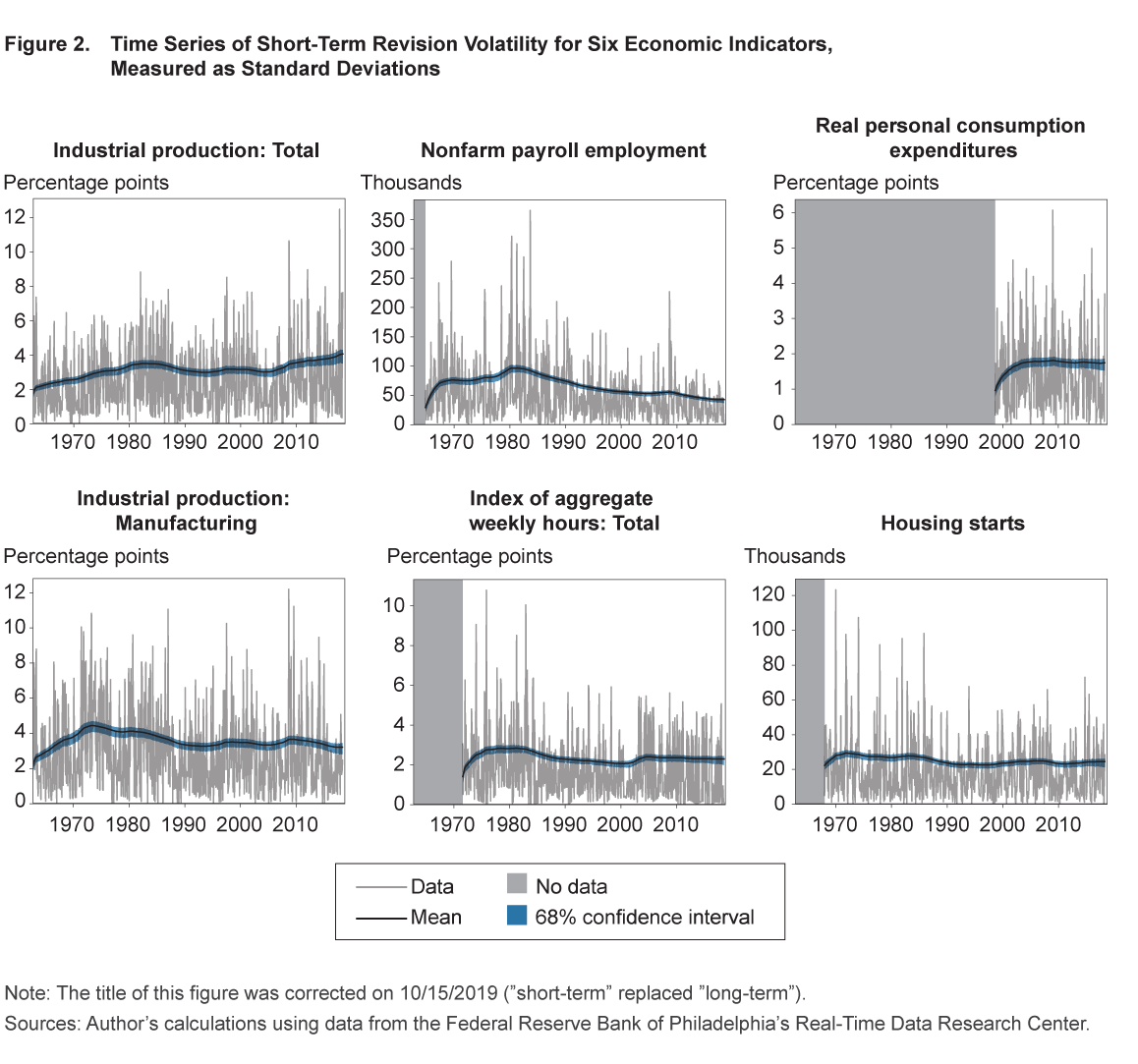
One can see that, after having controlled for the time-varying means, the volatilities of the revision processes are relatively stable over time for most series. There are two notable exceptions to this pattern.
First, the typical size of a revision to total IP has trended up over time. When the data sample begins, a one-standard-deviation revision to total IP growth is about 2 percentage points and by the end of the sample a one-standard-deviation revision to total IP growth is almost 4 percentage points. Interestingly, such a pattern is not present in the manufacturing IP data. While the first-second-third data do not contain the necessary detail to decompose the total IP revisions into subcomponents, it is worth noting that the composition of the industries in the IP series have changed over time. For example, the share of mining in total IP has more than doubled from 6.7 percent in the year 2000 to 14.6 percent in the year 2018. To the extent that activity in some industries is easier to measure in real time than others, changing industry composition can be a fundamental cause of time variation in the volatility of revisions.8 Of course, to whatever extent this changing composition is in fact statistically relevant, the models estimated here will uncover the effect.
Second, there has been a marked decline in the volatility of revisions to employment changes. Over the course of the sample, the volatility of employment changes has fallen almost by half, from a one-standard-deviation revision being about 100,000 workers in the early 1980s to a one-standard-deviation revision being about 50,000 workers at present. Hence, real-time data on employment changes have become appreciably more reliable than they were in the 1970s and 1980s.
Before examining the long-term revisions, I pause to take inventory of the key regularities of the short-term revisions uncovered by our time-series models. Namely, each indicator’s revision series examined here has tended to appear weaker in real time than it did with just a few months of hindsight. While the magnitude of the typical revision has been fairly stable over time, it is helpful for policymakers to know that the real-time data on total IP have become appreciably less reliable in the short term, while payroll employment data have become meaningfully more reliable. Of course, these results only describe how the economic picture has tended to change in the near term (relative to the initial release). The revision process can continue indefinitely, and so I next turn to examining the behavior of revisions that have occurred after the short term.
Results: Long-Term Revisions
Figure 3 shows the mean of the remaining cumulative revisions from the third release up to the current final release. As with the plots of short-term revisions, these charts show the revision data as well as the time-varying means and their 0.68 probability bands. In considering these results, it is important to keep in mind that they reflect additional revisions that occur only beyond the first-to-third revisions period analyzed in the previous section.
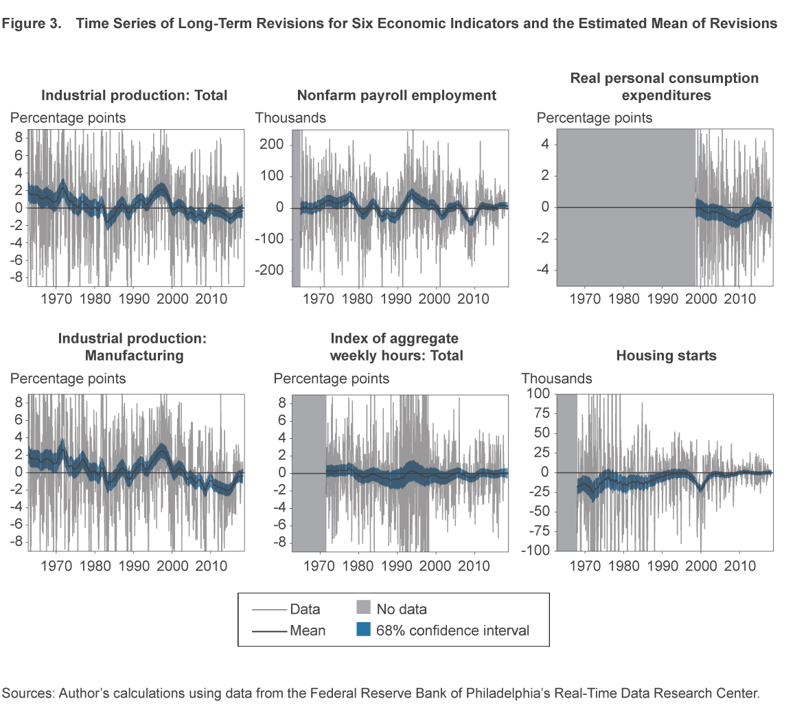
The salient features of these mean long-term revisions are more indicator-specific than for the short-term revisions; however, it is again by and large the case that the means show meaningful variation but without clear trends from the start of the sample to the present.
The one notable exception is with the revisions to housing starts, whose mean has trended from −25,000 housing units to essentially 0 at present, albeit with a few blips along the way.
Two of the indicators, real personal consumption expenditures growth and the change in hours worked, show little systematic bias at all in their long-term revisions; the 0.68 probability bands for the mean of these series typically include the value 0. This is not for a lack of meaningful revisions to the two series, as one can see from the revision data plotted along with the estimated time-varying means, but rather the revisions for the two series have been relatively idiosyncratic from one period to the next.
The growth rates of the IP series and changes to employment levels have seen meaningful variability in their mean long-term revisions over time, significantly larger in absolute value than their mean short-term revisions. As was the case for the short-term mean revisions, the mean revisions to total IP and manufacturing IP are near replicas of each other.
Last, I examine the standard deviation of the revision from the third-to-final release, shown in figure 4. The idea here is to present a measure of how much more information tends to be added later, after the “first, second, and third” cycle. To some degree, all of the figures show declining volatility of revisions over the sample. In other words, the older the data the larger in magnitude tends to be the revision up to the present. This is a reasonable result since observations closer to the present have had fewer opportunities to be revised. It is also implies a slightly more general statement for policymakers to be mindful of, namely that our knowledge of any given data point in an economic data series has continued to evolve indefinitely beyond the initial data release.
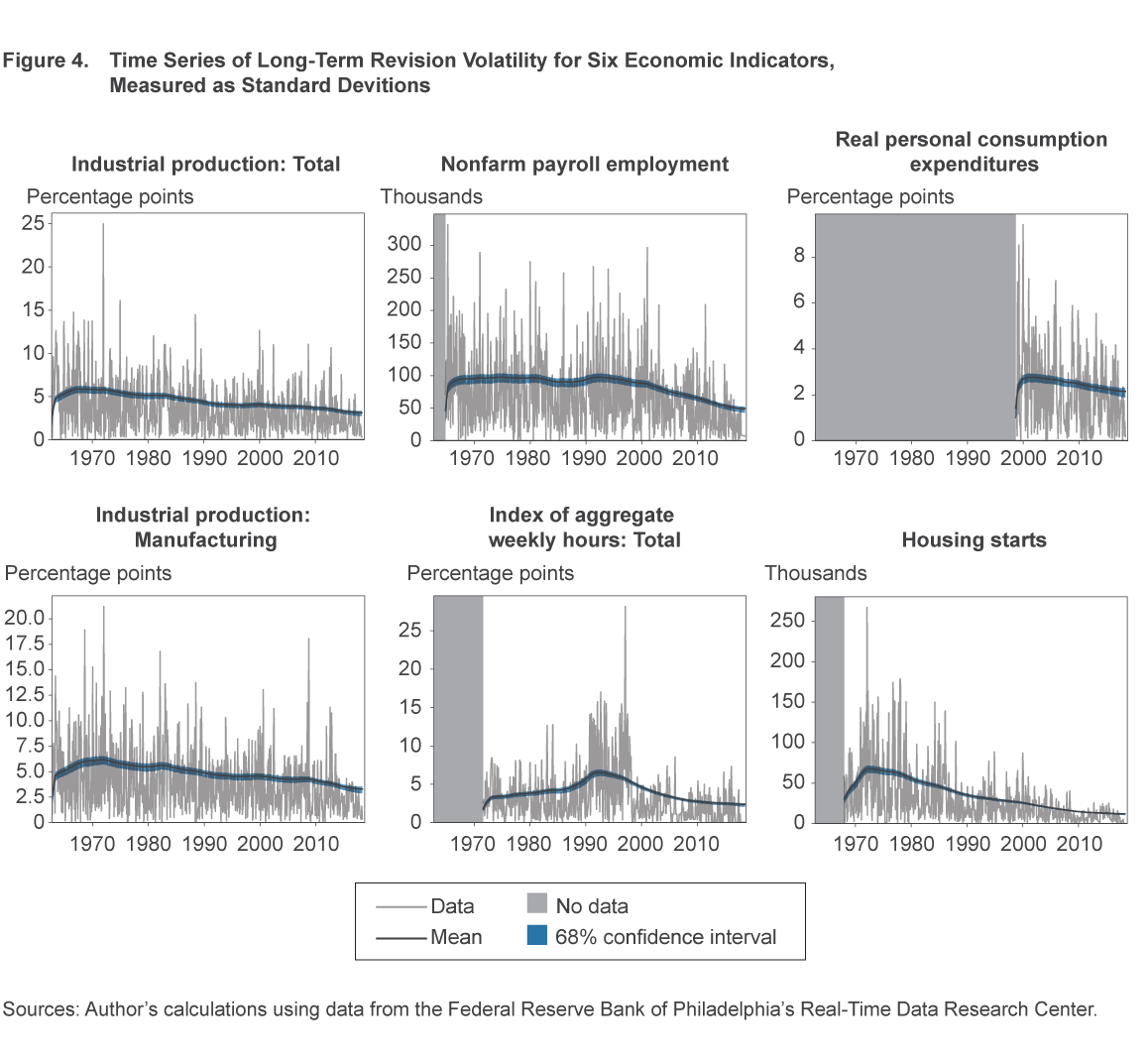
Furthermore, the estimated values in figure 4 are informative for how much our beliefs about the recent data are likely to change. By comparing figure 4 with figure 2, one can see that the cumulative revisions that occur after the “first, second, and third” cycle are typically at least as large as the first-to-third revisions. This observation suggests that, regardless of the vagaries of the short-term revision process, the view of the economy presented by these monthly indicators is likely not only to undergo changes well into the future, but substantial changes at that.
Conclusions
In this article I examined the extent to which the real-time reliability of six monthly macroeconomic indicators has remained stable over time by studying the time-series properties of their short-term and long-term revisions. The model estimates imply that both short-term and long-term revisions exhibit systematic deviations from zero that policymakers could build into their real-time assessments. Furthermore, some indicators’ revision series have seen substantial variation over time in the size of the typical revision, which suggests that some series have become less useful real-time indicators than they once were. Lastly, when examining the long-term revisions, it turns out that substantial revisions tend to occur indefinitely after the initial data release, a result which suggests a certain degree of caution is in order when using even thrice-revised monthly data in policymaking.
Footnotes
- The statistical properties of revisions have been examined in studies on real-time macroeconomic data. However, most previous studies have not examined the stability of revision properties over time. One exception is Aruoba (2008), who examines a number of properties of revisions across two different samples of data, one from before 1984 and another after 1984. Return to 1
- Some of the series analyzed in this article are subject to routine revisions beyond even the third release. For example, the value of the IP index in a particular month is subject to revisions in each of the five following monthly releases. Return to 2
- The exact share of the CES sample incorporated into the first, second, and third releases fluctuates over time, but, as a way to provide some context for typical values of the shares, note that over the period from 2008 to 2017 the average share incorporated into the “first preliminary release” was 74.1 percent, the average share for the “second preliminary release” was 92.4 percent, and the average share for the “third, final sample-based release” was 94.8 percent. More information on the revision process is available from the BLS at https://www.bls.gov/web/empsit/cestn.htm#section7a, and a detailed history of sample collection rates can be found at this BLS page. Return to 3
- See https://www.federalreserve.gov/releases/g17/ASA_paper_final.pdf. Return to 4
- In practice, data considered sufficiently old may not get revised. For example, the 2018 annual revision to IP did not alter the values of IP growth prior to 1972. See footnote 1 on this release. Return to 5
- The data are publicly available and can be downloaded from https://www.philadelphiafed.org/research-and-data/real-time-center/real-time-data/data-files. Return to 6
- The notion of probability used here is Bayesian, but the probability statement has some similarities to that which would accompany a Frequentist confidence set. Return to 7
- Industry compositions can be systematically found in “Table 4 Industrial Production Indexes: Market and Industry Group Summary” of the Industrial Production releases from February 2001 (January 2001 reference period) onward. The tables are available at https://www.federalreserve.gov/releases/g17/Current/default.htm. Return to 8
References
- Aruoba, S. Borağan. 2008. “Data Revisions Are Not Well-Behaved.” Journal of Money, Credit, and Banking, 40(2), 319–340.
- Bognanni, Mark. 2018. “A Class of Time-Varying Parameter Structural VARs for Inference under Exact or Set Identification.” Federal Reserve Bank of Cleveland, Working Paper No. 18-11.
Suggested Citation
Bognanni, Mark. 2019. “Has the Real-Time Reliability of Monthly Indicators Changed over Time?” Federal Reserve Bank of Cleveland, Economic Commentary 2019-16. https://doi.org/10.26509/frbc-ec-201916
This work by Federal Reserve Bank of Cleveland is licensed under Creative Commons Attribution-NonCommercial 4.0 International

