

- Share
New Data on Wealth Mobility and Their Impact on Models of Inequality
Using data on families’ wealth over time, we calculate changes in relative wealth mobility; that is, how likely families are to move up or down the wealth distribution, relative to one another. We find families have become less likely to change their position in the wealth distribution over time, and those that do move are less likely to go very far. We also look at the savings behaviors that are associated with more mobile families and find that families that make large movements through the wealth distribution appear to be more likely to own some form of a risky asset.

The views authors express in Economic Commentary are theirs and not necessarily those of the Federal Reserve Bank of Cleveland or the Board of Governors of the Federal Reserve System. The series editor is Tasia Hane. This paper and its data are subject to revision; please visit clevelandfed.org for updates.
Wealth inequality, the unequal distribution of assets across households, has been rising for decades. However, this statistic alone gives an incomplete picture of the inequality of households’ economic experiences and opportunities. A fuller understanding comes from also knowing how much movement within the distribution households experience over time. For instance, is it likely that someone with low wealth today will be a wealthy person at some point in the future, or are they rigidly stuck at the bottom? In other words, a fuller understanding of households’ economic
opportunity comes from a combination of data on both wealth inequality and wealth mobility.
This Commentary explores the topic of wealth mobility in the United States during the past three decades (see Carroll and Chen 2016 for similar work on income inequality and mobility). Examining supplemental data from the Panel Study of Income Dynamics (PSID), which track families’ wealth over time, we calculate changes in relative wealth mobility; that is, how likely families are to move up or down the wealth distribution, relative to one another. We find that wealth mobility has declined since the 1980s, a trend that is robust to a wide range of measures. Finally, we identify savings behaviors that are associated with more mobile families. Such behaviors may explain the disparity between observed levels of mobility and the levels predicted by the standard model used to study inequality.
Determinants of Wealth Mobility
Households move up and down the wealth distribution for many reasons. Households’ savings behavior is one factor that affects their mobility. For example, those who hold portfolios composed primarily of riskier, but higher-expected-return assets (such as stocks) are more likely to move up or down in their wealth position than those who hold less risky assets (such as savings bonds). Marriage and divorce, which may lead to assets being combined or separated, can cause large movements upward and downward, respectively.
Other factors may be driven greatly by luck. Did a risky asset return a high payoff, or did it fail? Was the household subject to expensive medical bills due to an unforeseenillness? Did the household receive a large bequest from a parent? In some cases, it may be a mix of both luck and choice, as in the case of a bankruptcy.
Age can also affect mobility. Household savings behavior follows a “life cycle.” Young households are generally more wealth-poor because they have had little time to save. They often borrow (in anticipation of future labor income) to make large purchases such as a car, a house, or an education. As a result, they tend to start out low in the wealth distribution. As households age, they typically save more, paying down debt and building up a retirement fund, so they rise in the distribution. Finally, when households enter the retirement phase, they dissave, dipping into their accumulated wealth to fund consumption. This drawing down of savings moves households back down the wealth distribution over time.
Measuring Wealth Mobility
Since 1984, the PSID has included a wealth module that attempts to measure the evolution of household wealth. In order to get a comprehensive estimate of wealth, interviewers ask participants a series of questions that separate total net worth into nine subcomponents. These include equity in the main family home and a wide variety of investments, ownership equity in a farm or business, and all outstanding debt outside of a mortgage or auto loan. The PSID then calculates two values for family net worth: one which includes all nine components, and another which excludes equity in the main home. Because homes are a major savings vehicle, and thus one of the primary means by which households can change their wealth, we choose the measure that includes home equity. In order to compare wealth across time, we use the consumer price index (CPI) to convert all values to constant 2016 dollars.
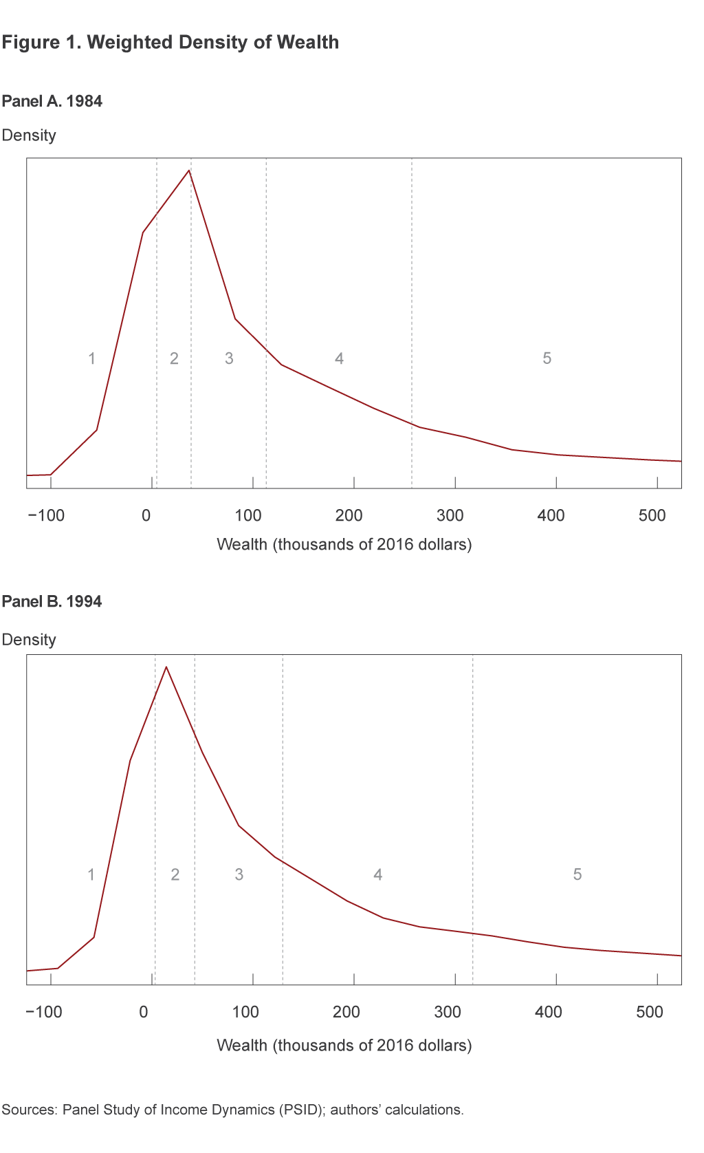
We examine eight releases of the PSID and track family wealth over 10-year increments beginning in 1984 and ending in 2013. The increments are 1984–1994, 1994–2003, 2003–2013. By comparing a family’s position in the wealth distribution at the beginning of the sample to its position at the end of it, we can compute wealth mobility. For example, let’s say we begin in 1984. We would construct the wealth distribution of the panel in that year and then divide it into equally populated bins. The first bin is the poorest, the second the next poorest, and so on up to the final bin, which contains the wealthiest families in the data. For this analysis, we divide the distribution into quintiles, meaning that there are five bins, and each bin contains 20 percent of the population. Then we look at the wealth distribution of the panel 10 years later and divide it into quintiles. Figure 1 plots these wealth distributions for 1984 and 1994 along with their respective quintiles. The dashed lines indicate the wealth-level cutoffs that separate each of the bins.
Because the PSID is a panel, we can see which quintile any family starts in and which quintile it ends up in. From this we can calculate, for example, the fraction of families among the poorest 20 percent in 1984 who were among the richest 20 percent in 1994. By constructing these fractions for every possible quintile combination (first to the fifth, second to the third, fourth to the first, etc.), we construct a mobility matrix or table. The rows indicate the initial quintile and the columns indicate the final quintile.
Table 1 presents the mobility matrix for US households from 1984 to 1994. According to the table, approximately63 percent of sample households who were in the first quintile in 1984 were also in the first quintile in 1994, while slightly less than 2 percent transitioned to the fifth quintile.
1. Wealth Mobility Matrix
| Quintile in 1994 | ||||||
|---|---|---|---|---|---|---|
| 1 | 2 | 3 | 4 | 5 | ||
| Quintile in 1984 | 1 | 0.629 | 0.234 | 0.087 | 0.026 | 0.018 |
| 2 | 0.229 | 0.413 | 0.214 | 0.098 | 0.047 | |
| 3 | 0.100 | 0.276 | 0.326 | 0.206 | 0.092 | |
| 4 | 0.053 | 0.083 | 0.263 | 0.371 | 0.229 | |
| 5 | 0.017 | 0.034 | 0.088 | 0.252 | 0.609 | |
Sources: Panel Study of Income Dynamics (PSID); Carroll, Hoffman, and Young (2017).
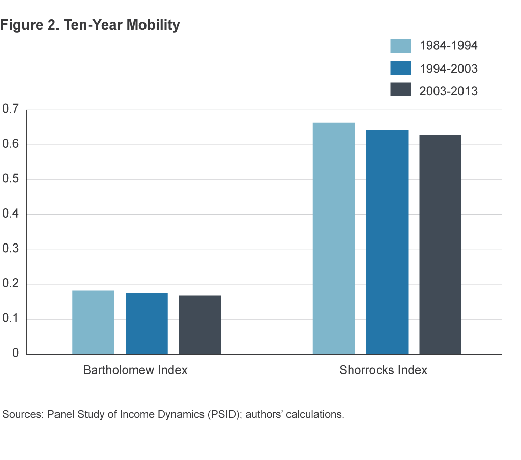
The information in the mobility matrix can be summarized using a single number between zero and one. Zero corresponds to the least possible degree of mobility, and one corresponds to the maximum degree. Different measures summarize the information differently, varying in the emphasis they place on various features of the matrix. For example, the Shorrocks index indicates how likely a household is to remain in the same quintile across time. This measure does not account for the distance moved. The Bartholomew index, on the other hand, weights more heavily movements that cross over multiple quintiles. This latter measure strikes a balance between the frequency of movement and the distance moved. For details on how each index is constructed as well as results from other measures, see Carroll, Hoffman, and Young (2017).
Figure 2 plots wealth mobility measured in each of the three 10-year periods studied. Irrespective of the measure chosen, the data indicate that wealth mobility has decreased over the past three decades. On average, households are now more likely to remain in the same wealth quintile over 10-year periods than they were two decades ago (Shorrocks index) and less likely to experience large movements across quintiles (Bartholomew index). For instance, the percentage of households that stayed in the top quintile from 2003 to 2013 was 7 percentage points larger than the percentage of households that stayed in the top between 1984 and 1994. Perhaps surprisingly, the same comparison of households in the bottom quintile showed a 6 percentage point decline, meaning households got out of the bottom quintile moreoften between 2003 and 2013 than they did between 1984 and 1994. Nevertheless, the probability that a household outside of the top quintile transitioned into it within 10 years was roughly half as likely between 2003 and 2013as between 1984 and 1994.
Is It Structure or Exchange?
While wealth mobility differs from wealth inequality, the latter can affect the former. Rising wealth inequality spreads households farther apart in terms of wealth, and this spreading out can increase the distance covered by each bin. The increase in wealth inequality is shown in Figure 1. Notice that the wealth levels that demarcate the third, fourth, and fifth quintiles in 1994 are farther to the right (higher wealth) than those in 1984. In other words, it took a higher relative income for a family to make it into these upper quintiles in 1994 than it did in 1984. We call this stretching out of wealth cutoffs a change in the structure, or shape, of the distribution.
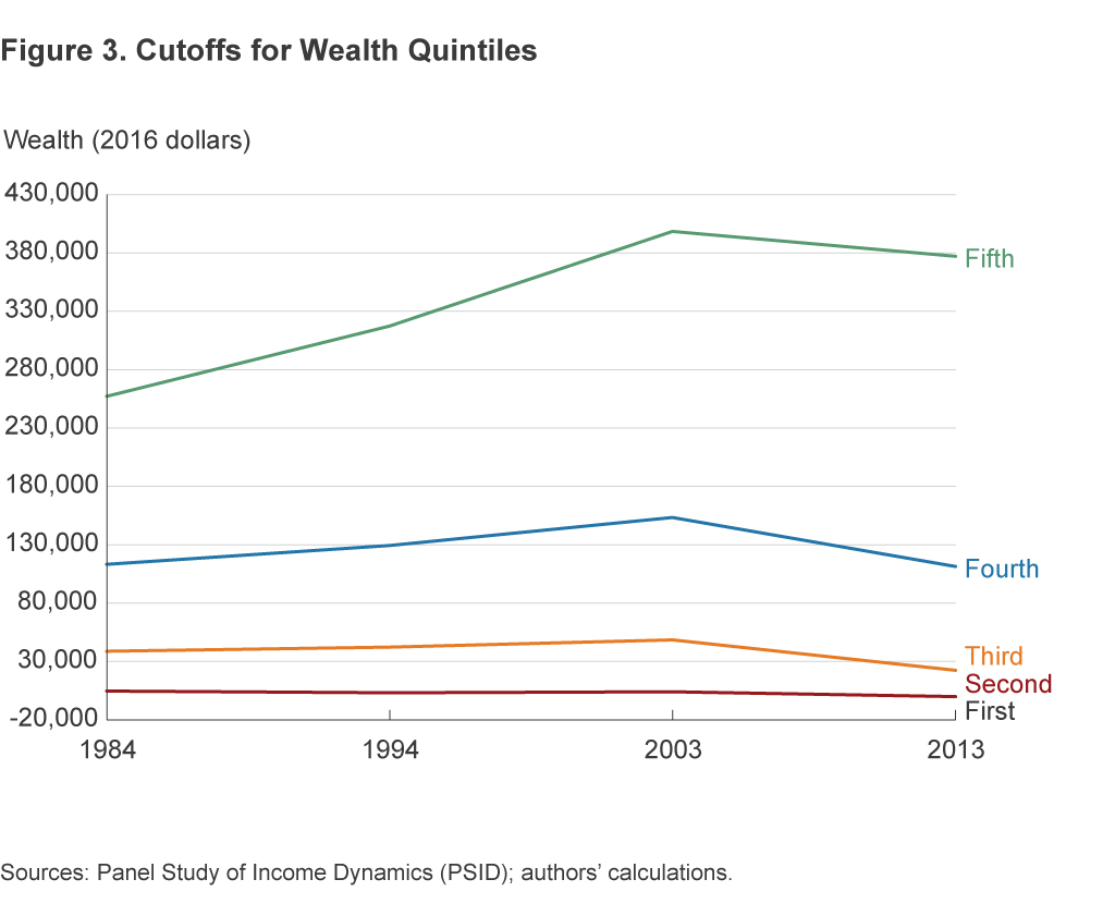
Figure 3 plots the amount of wealth needed to cross into each quintile. Over the period studied, the threshold between the first and second quintiles has held steady near zero wealth. The other thresholds increased through most of the sample, especially the one defining the top 20 percent. Even at the end of the sample (2003–2013), when all cutoff levels declined, the spread between the top two thresholds expanded. When the amount of wealth required to be part of the top 20 percent increases, it is harder, all else equal, for poor households to reach the top bin. Thus, poor households will transition into the top quintile less frequently, and this will appear as a decrease in mobility, even though nothing may have changed about these households’ saving behavior.
The change in the value of a mobility measure that is due solely to the stretching of the distribution is called structural mobility. As the name implies, it captures movements in measured mobility that are induced by changes in the structure of the distribution. The portion of the change in measured mobility that cannot be attributed to structural mobility is called exchange mobility. It captures how frequently households move between bins when the size of the bins remains fixed over time.
How much of the reduction in wealth mobility observed in the data can be accounted for by the rise in wealth inequality? To answer this, we look at the same households over 10-year samples, but instead of adjusting the wealth thresholds from the original year to the final year as before, we leave them unchanged. This keeps the wealth threshold between quintiles constant over the measurement period and removes any mobility due to changes in the shape or structure of the wealth distribution. The decomposition of total mobility into exchange and structure is presented for both the Bartholomew index and the Shorrocks index of mobility in Figures 4 and 5.
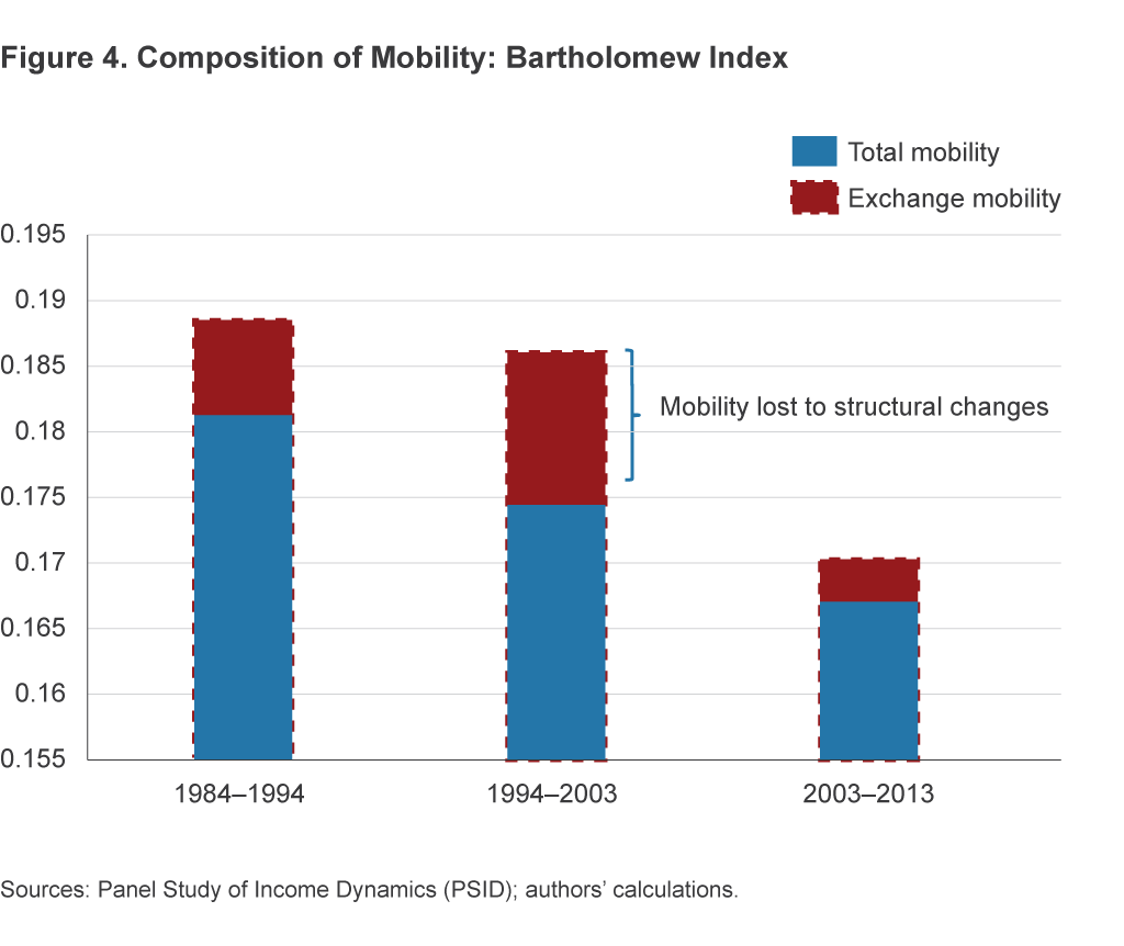
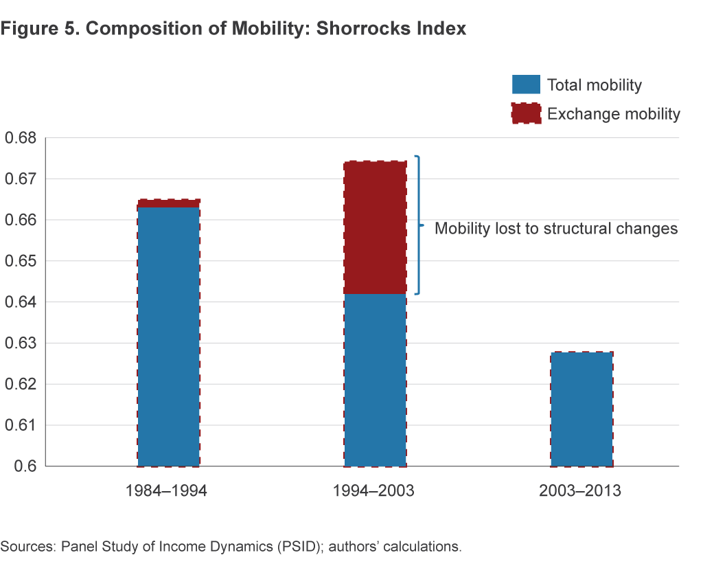
While rising wealth inequality is not the only factor in the decline in wealth mobility, the broad pattern is that households are relatively less likely to move, even given a fixed distribution. The structural component accounts for roughly 5 percent of the decline in the Shorrocks index and 22 percent of the decline in the Bartholomew index. In addition, the Shorrocks index shows that mobility would have increased in the 1994–2003 sample if wealth inequality had remained the same (instead of growing).
Note that the differences in the way the two indicators measure mobility lead to a considerable difference in the way they decompose the change in mobility into structure and exchange. Rising wealth inequality played only a modest role in limiting the probability of families exiting their initial wealth quintile (Shorrocks), but it had a much larger effect on the likelihood that a household ended in a more distant quintile (Bartholomew). In other words, families were only slightly less likely to move, but much less likely to move very far.
Aligning Macroeconomic Models with Data on Mobility
Economists employ macroeconomic models to evaluate the effects that changes in the economy or changes to policy might have on inequality. Many of the conclusions reached in those models depend on the model’s assumptions about wealth mobility. Recent research suggests that the assumptions made in the standard model of inequality are not consistent with the data on mobility. Carroll, Hoffman, and Young (2017) find that the model’s baseline specification implies far less wealth mobility than the data do. Table 2 shows measures of mobility in the model and the PSID data. The ranges of measures in the model arise from varying model parameters, while the ranges in the data come from variations in mobility over time, as measured in the PSID wealth data.
2. Wealth Mobility (Model vs. Data)
| Index | Range in model | Range in data |
|---|---|---|
| Bartholomew | 0.017–0.074 | 0.138–0.155 |
| Shorrocks | 0.086–0.368 | 0.555–0.608 |
Sources: Panel Study of Income Dynamics (PSID); Carroll, Hoffman, and Young (2017).
Further, Carroll, Hoffman, and Young show that while there are variations of the model that can produce the amount of upward mobility observed in the data, they still fall short in delivering the right amount of downward mobility.
We study the PSID data again to look for features that could be added to the model to better account for these large movements. We isolate households that move three or more quintiles. These households either go from being among the poorest to being among the richest or frombeing among the richest to being among the poorest within 10 years. We call these households “jumpers” and compare their behavior with nonjumpers to identify any patterns that could explain the jumper’s large wealth movements.
Our results suggest that for the 2003–2013 period, one of the main characteristics that differentiates jumpers and nonjumpers was their relative tendencies to own higher-risk assets, such as volatile investments, real estate other than their own homes, a farm, or a business. We measure these tendencies as the likelihood that a given family indicated ownership of any such asset at least once during the sample horizon. Figure 6 shows these results for the period.1
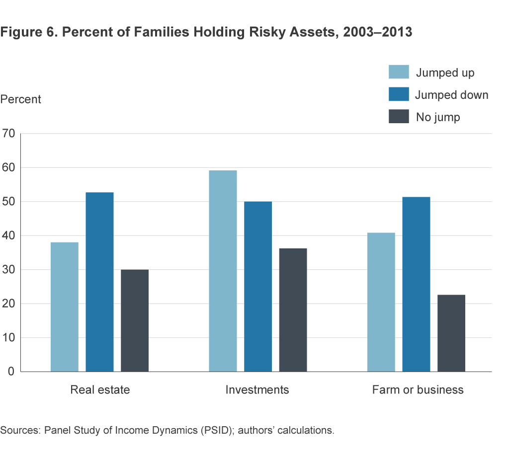
Notably, an increased tendency to own a risky asset was a hallmark both of families that moved up three or more quintiles and of those that moved down three or more quintiles. An example of the discrepancy between families that jumped and those that did not is in the ownership of a farm or business: 41 percent of families that jumped up and 51 percent those that jumped down reported owning such an asset, as compared to just under 23 percent of families that did not make a jump. These statistics suggest that the same types of behaviors contribute to both large upward and large downward movements. Families that take on the risk of investing in stocks or real estate, or owning a farm or business, face the potential for a large payoff (which would move them upward quickly in the distribution) or a large loss (which would move them downward quickly in the distribution).
Conclusion
Wealth mobility depends on luck and household choices. It is a reflection of households’ opportunities as well as their responses to those opportunities. Panel data from the past 30 years show a decline in wealth mobility across several measures. It appears that families are less likely to change wealth quintiles over time, while those that do move are less likely to move very far. The reasons for these trends are not fully known, but increasing wealth inequality has contributed to the decline. Families that do make large movements through the wealth distribution appear to be more likely to own some form of a risky asset, as compared to families that do not make large movements.
Economists are coming to a better understanding of wealth mobility, and this understanding will lead to better models. In the meantime, it is helpful to keep these mobility trends in mind when interpreting new information about wealth inequality.
Footnotes
- Similar trends are evident in the 1994–2003 sample. Return to 1
References
- Carroll, Daniel R., and Anne Chen, 2016. “Income Inequality Matters, but Mobility Is Just as Important,” Federal Reserve Bank of Cleveland, Economic Commentary, no. 2016-06.
- Carroll, Daniel R., Nicholas Hoffman, and Eric R. Young, 2017. “Mobility,” Federal Reserve Bank of Cleveland, Working Paper no. 16-34R (forthcoming).
Suggested Citation
Carroll, Daniel R., and Nicholas Hoffman. 2017. “New Data on Wealth Mobility and Their Impact on Models of Inequality.” Federal Reserve Bank of Cleveland, Economic Commentary 2017-09. https://doi.org/10.26509/frbc-ec-201709
This work by Federal Reserve Bank of Cleveland is licensed under Creative Commons Attribution-NonCommercial 4.0 International

