I thank Keith Kuester and Jürgen von Hagen for inviting me to participate in the Konstanz Seminar on Monetary Theory and Monetary Policy. I am happy to be here for a number of reasons. First, I remember very fondly hiring Keith when I was research director at the Federal Reserve Bank of Philadelphia. Keith was a very productive addition to our department. While I was sad to see him eventually return to Germany, I was very thankful we were able to learn from Keith during his time with us. And hopefully, he was able to learn a little bit from his Fed colleagues as well.

A second reason I am happy to be here is that it is a great honor to contribute to a forum that for more than four decades has fostered a fruitful dialogue between academic researchers and policymakers on both sides of the Atlantic. In the published proceedings of the first conference held in 1970, the seminar’s founder, Karl Brunner, provided the insight that “theory without application to our environment is useless and policy discussion or judgments not based on analysis are dangerous.”¹ I believe that Professor Brunner would be very gratified by the discussions over the past two days, which have better joined monetary theory and monetary policy.

Today, I’d like to spend some time talking about inflation. But before I do, I should mention that these are my own views and not necessarily those of the Federal Reserve System or my colleagues on the Federal Open Market Committee.

It seems clear to me that if there is one topic that would benefit from better understanding the interplay of theory and policy, it is inflation. For a monetary policymaker, price stability is the Holy Grail — price stability is the one thing that monetary policy can ensure over the longer run, and monetary policy is the only tool that can ensure price stability over the longer run. The benefits of price stability for the economy are clear.² Stable prices mean businesses and households don’t have to spend time trying to protect the purchasing power of their money; they can make long-term plans and commitments without having to deal with the uncertainty about the value of their money. When the price level is stable, any price changes reflect changes in the supplies of certain goods or services relative to others and this information is helpful to businesses and consumers when they have to allocate their scarce resources. Price stability also promotes other goals like financial stability and confidence in the economy, thereby supporting growth and maximum employment, the other part of the Federal Reserve’s dual mandate.

While price stability and monetary policy are intimately linked, setting monetary policy to achieve price stability is not trivial. It requires being able to measure inflation so that we’ll know how far we are from the goal. It requires being able to forecast inflation because monetary policy affects the economy with a lag that varies over time and with economic circumstances. It requires understanding the determinants of the monetary policy transmission mechanism. And it also requires having the wherewithal to make decisions under uncertainty. Given the importance of understanding inflation for monetary policy, one could get pretty discouraged about the state of our knowledge — I admit that sometimes such thoughts come to me, usually late at night. But instead of turning nihilistic, I think it’s better to keep pushing the envelope of our knowledge outward, as central bank and academic researchers are doing, and to learn to deal with the uncertainty as best we can. Before I discuss some of the advances being made and some open issues, let me review recent inflation developments.

Recent Inflation Developments

Many central banks conduct monetary policy with a goal of achieving an explicit inflation target. Such an explicit target provides transparency to the public and helps anchor expectations about inflation. When businesses and consumers have confidence that the central bank is committed to its goal over the longer run and will defend the target, they are more likely to look through temporary changes in inflation. Although it was discussed at various times over the years, the Federal Reserve’s Federal Open Market Committee (FOMC) established its explicit inflation target relatively recently, in January 2012, when it issued its statement on longer-run goals and monetary policy strategy. The FOMC’s inflation goal is 2 percent, as measured by the year-over-year change in the price index for personal consumption expenditures, or PCE inflation. As indicated in its annual reaffirmation of this goal in January of this year, the FOMC views this goal as symmetric. That is, the FOMC would be concerned if inflation were running persistently above the objective, and also if it were running persistently below its objective. By helping Fed policymakers set appropriate monetary policy, the explicit 2 percent inflation target promotes not only price stability but also maximum employment.

The Federal Reserve has not always been successful at achieving price stability. There have been misses on both sides. During the Great Depression in the 1930s, the U.S. experienced deflation. In the aftermath of the oil price shocks in the 1970s, inflation surged and remained high until then-Fed Chairman Paul Volcker began to tighten monetary policy to bring inflation down, at the cost of a deep recession in the early 1980s. These periods point out the importance of a central bank remaining focused on its price stability goal, because when attention wanders, there are severe costs to consumers and businesses.

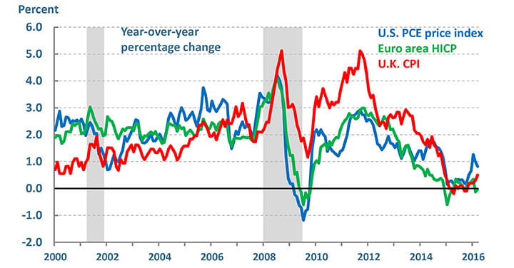
Relative to the Fed’s 2 percent goal, inflation has been low for quite some time, and while the most recent data are encouraging and consistent with the FOMC’s view that inflation will gradually move back to target over time, a reading of FOMC statements since the Great Recession clearly shows that inflation has been a focus of the Committee. As shown in Figure 1, low inflation has been a phenomenon not only in the U.S. In recent years, inflation has also run well below the United Kingdom’s 2 percent inflation target, as measured by the consumer price index (CPI), and the European Central Bank’s inflation target of below, but close to, 2 percent, as measured by the changes in the harmonized index of consumer prices (HICP). By each central bank’s respective target index, last year, inflation was 0.20 percent in the U.K., 0.25 percent in the Euro area, and 0.66 percent in the U.S.

A couple of common factors have contributed to the low inflation rates in these countries in recent years. First, in the aftermath of the financial crisis and during the slow recovery from the Great Recession, global demand was weak. Indeed, over the 2009-2011 period, one puzzle for policymakers was actually not why inflation was low, but rather, why it wasn’t lower.³ More recently, inflation has been kept down by the decline in energy and other commodity prices, and in the U.S., a rise in the value of the dollar, which puts downward pressure on the prices of imports into the U.S. According to dynamic simulations of the Board of Governors staff’s SIGMA model, a 10 percent rise in the real value of the dollar affects core inflation via import prices fairly quickly, resulting in a drop of about 0.5 percent in core inflation a year after the shock, which partially reverses over the subsequent year. A shock to the value of the dollar also tends to reduce GDP with a lag, and the model indicates that this would put additional downward pressure on inflation.⁴

Of course, growth, commodity price changes, and currency fluctuations are not necessarily independent events. For example, a portion of the over 60 percent decline in oil prices since mid-2014 likely reflects expectations of weaker growth in China and other countries, although supply factors likely play a greater role. Similarly, since mid-2014 the U.S. dollar has appreciated almost 20 percent, reflecting expectations that real growth in the U.S. will continue to be stronger than growth abroad, as well as projected interest rate differentials between the U.S. and other economies. So we have to be careful about thinking of these shocks as independent and just summing their effects.

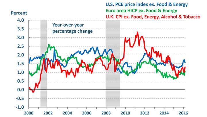
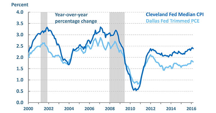
In trying to assess current and projected inflation, economists often look at measures of underlying inflation to get a sense of the trend. Some of these measures, like core inflation, shown in Figure 2, delete food and energy prices because they tend to be volatile. Other measures, like the Cleveland Fed’s median consumer price index, or the Dallas Fed’s trimmed-mean PCE inflation rate (shown in Figure 3), are constructed to reduce the influence of those components that have shown outsized changes; the particular components can vary from month to month.

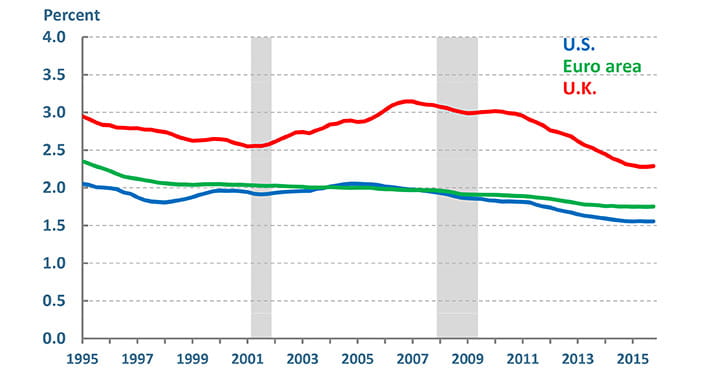
Economists also use various models to get a sense of the underlying trend in inflation. Figure 4 shows estimates of trend inflation for the U.S., Euro area, and U.K. based on an autoregressive model that allows continuous time variation in coefficients and the variance of shocks to inflation.⁵ Based on this model, as actual inflation rates have declined, estimated trend inflation has also declined modestly in each location. The Cleveland Fed staff has estimated several different models of trend inflation for the U.S., and they also exhibit declines in the trend over the past decade, suggesting that the result is not model specific.⁶

Of course, the estimates do not mean that the change in trend is a permanent one, with inflation mired below target. In fact, in the U.S., as oil prices and the dollar have shown some stability of late, the headline and underlying measures of inflation have moved higher, in accordance with the pattern anticipated by the FOMC. As of the first quarter of this year, the year-over-year change in the headline PCE price index has risen to 1 percent from 0.2 percent in the first quarter of last year. Core PCE inflation was 1.7 percent in the first quarter, compared to 1.3 percent a year ago, and core CPI inflation was 2.3 percent compared with 1.7 percent a year ago. The 12-month change in the Cleveland Fed’s median CPI inflation rate averaged 2.4 percent in the first quarter, and it, too, has been rising over the past year.

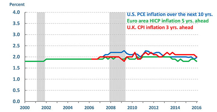
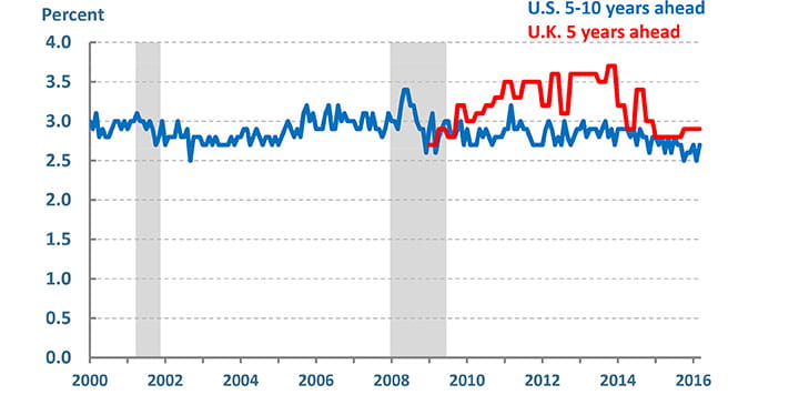
Inflation expectations are an important determinant of inflation dynamics.⁷ There are a variety of ways to measure inflation expectations. Some measures are based on surveys of households or of professional economic forecasters; others are derived from transactions in financial markets. In my view, looking across measures, inflation expectations over the past few years have been relatively stable, even in the face of sizable declines in energy prices. This stability is most readily apparent in the survey measures of longer-term inflation expectations of professional forecasters, as seen in Figure 5. But it is also seen in survey measures of household expectations, depicted in Figure 6. Although these are measures of longer-term inflation expectations, analysis suggests household inflation expectations are sensitive to large changes in energy prices, and so the slight move down in the U.S. since mid-2014 may reflect the sharp decline in oil prices.⁸

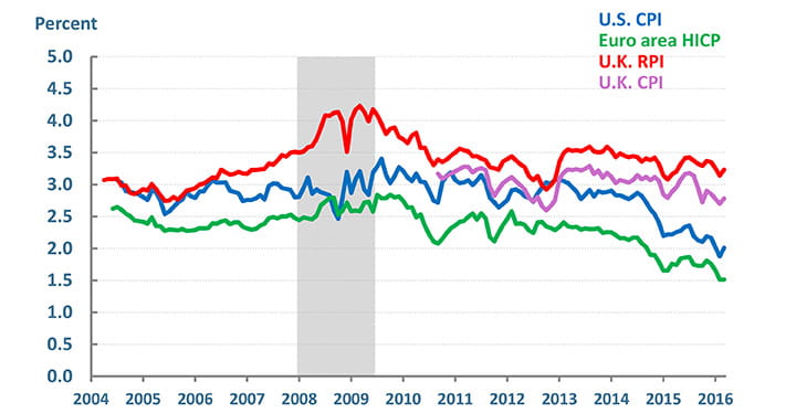
To augment the survey measures, economists have also developed models to derive inflation expectations from financial market data. In the U.S., the 10-year breakeven inflation rate is measured by the difference between the yield on 10-year Treasuries and the yield on 10-year Treasury inflation-protected securities (TIPS). The U.S. Treasury began issuing TIPS in 1997 to allow investors to take out some insurance against unanticipated changes in CPI inflation. Theoretically, inflation swaps offer a similar way for investors to protect themselves. Inflation compensation based on swaps is another measure commonly used as an indicator of inflation expectations. These market-based measures can be volatile. Figure 7 shows five-year inflation compensation five years ahead — the so-called five-year, five-year forward measure. I am smoothing through some of the volatility and showing monthly data. As you can see, over the past two years, the measures have declined a bit in the U.S. and in the Euro area.

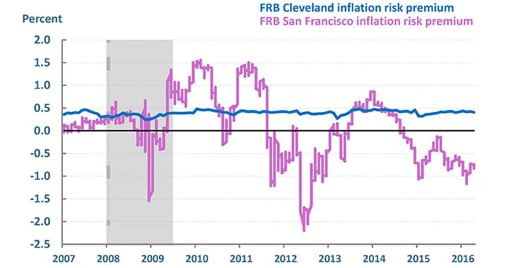
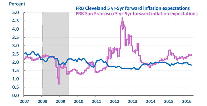
One needs to remember that there are differences between inflation compensation and inflation expectations. In particular, the inflation compensation measures reflect not only investors’ expectations about inflation but also the amount they are willing to pay in order to protect themselves from inflation risk. In addition, the TIPS market is less liquid than the Treasury market, so there is a liquidity premium in inflation breakeven and compensation rates. We should expect the inflation risk premium and the liquidity premium to vary over time, so one needs to use a model to extract a measure of inflation expectations from inflation compensation. These models can produce very different estimates of the components depending on circumstances. For example, Figure 8 shows the inflation risk premia based on models maintained by the Cleveland Fed staff and the San Francisco Fed staff.⁹ You’ll note that even the signs can differ: in the most recent period, the San Francisco Fed model is estimating a negative risk premium while the Cleveland Fed model is estimating a positive risk premium. So the inflation expectations derived from these models can be quite different, as shown in Figure 9. In addition, at times, demand for Treasuries can increase significantly as investors seek safe haven flows for their money. This can make it even harder to infer inflation expectations from changes in inflation compensation. Finally, in the U.S., changes in the inflation compensation measures also seem to be correlated with changes in energy prices, a correlation that suggests they may not be reliable indicators of long-term inflation expectations.

Jon Faust and Jonathan Wright argue that market-based inflation compensation measures are too volatile to be plausible estimates of longer-term inflation expectations, and they show that the data reject the hypothesis that today’s five-year, five-year forward inflation compensation is a rational expectation of inflation in the long-run.¹⁰

Given the measurement challenges and the volatility we saw in financial markets last summer and at the turn of the year, I think we need to be somewhat cautious when inferring a signal about changes in inflation expectations from these market measures. Nonetheless, I also think it is worth monitoring all of the available indicators of inflation expectations because of the important role expectations play in inflation dynamics.

Inflation Models and Forecasts

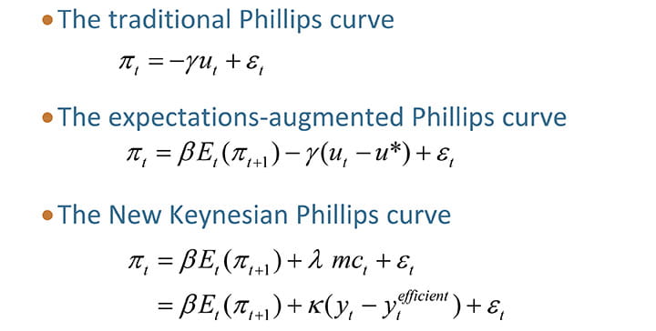
The factors I’ve discussed — demand growth, oil and other relative price shocks, and inflation expectations — are factors that appear in the expectations-augmented Phillips curve, a statistical relationship that economists use in forecasting inflation (Figure 10). While the original version of the Phillips curve related changes in inflation to changes in unemployment, the newer version stresses the importance of inflation expectations in inflation dynamics and puts less emphasis on measures of economic activity. It generally provides better inflation forecasts than the traditional Phillips curve.

In the expectations-augmented Phillips curve, economic activity is represented by a measure of slack — usually either the unemployment gap, which is the deviation of the unemployment rate from its longer-run natural rate, or the output gap, which is the deviation of output from its longer-run trend or potential level. A body of research has found that the estimate of the slope coefficient on slack in the expectations-augmented Phillips curve has diminished and that inflation expectations are a more important driver of inflation dynamics. In terms of forecasting ability, the model’s under-prediction of inflation in the early stages of the recovery in 2009-2011 renewed questions about the reliability of the Phillips curve in forecasting inflation. This generated a considerable amount of investigation aimed at resolving the puzzle of the missing disinflation. Analysis by economists at the ECB indicates that including food and energy prices in the Phillips curve for core inflation can explain the missing disinflation in the Euro area between 2009 and 2011.¹¹ This points out that how the Phillips curve is specified and the measures one uses for inflation expectations and economic slack are likely to affect its forecasting ability — which doesn’t offer much solace if one wants to use the model in real time.

More than that, we need to acknowledge that the measures of slack in the Phillips curve relationship are imprecise because they depend on unobservables like the natural rate of unemployment and the level of potential GDP. The slack measures also get revised over time. In fact, economists have been revising down their estimates of potential growth almost every year since the Great Recession started. For example, in 2008, the Congressional Budget Office estimated that potential growth between 2008 and 2013 would average 2.5 percent, well above its current estimate of 1.3 percent for that same time period. Revisions also plague certain inflation measures, like PCE inflation in the U.S., which complicates making monetary policy in real time. For example, in early 2002, FOMC policymakers were concerned about a drop in inflation. Ultimately, much of this drop was revised away. In a number of papers, Athanasios Orphanides has laid out a convincing case that mismeasurement of slack and other unobservables like the natural rate of interest led to monetary policy mistakes that contributed to the Great Inflation of the 1970s. He argues that these mismeasured concepts continue to unduly influence monetary policy today.¹²

The New Keynesian Phillips curve is an alternative to the statistical Phillips curve I have been discussing. It is a component of the dynamic stochastic general equilibrium (DSGE) model, the workhorse model in wide use at central banks. The model assumes that firms have some pricing power, i.e., there is imperfect competition, and a firm will set its price in order to maximize its profit. But the model also assumes that prices are sticky, i.e., the firms can adjust their prices only infrequently and not with every shock that hits the economy. These distortions mean that when the economy is hit by a shock, the level of output can differ from the efficient level that would prevail in the absence of sticky prices and with perfect competition. They also mean that monetary policy can affect real activity in the short run, even though it has a neutral effect on real activity in the long run, and that the main driver of inflation dynamics in the short run is the expected markup over marginal cost that firms charge to their customers. This expected markup will vary over time and economic circumstances.¹³

One implication of the New Keynesian Phillips curve is that the usual measures of economic slack play a role in inflation dynamics only to the extent that they help predict future changes in marginal costs, which does not seem to be the case. However, there is a different concept of slack that appears in the New Keynesian Phillips curve. The relevant measure of slack is the difference between the efficient level of output and the prevailing level of output in the economy with its sticky prices and imperfect competition. Inflation, then, is related to expected inflation and this gap. In the absence of shocks that affect the firms’ desired markups of price over marginal cost, monetary policy should seek to minimize this gap, which would be equivalent to stabilizing inflation. The nature of the shock hitting the economy will determine whether the efficient level of output will change and whether monetary policy will want to respond to it.

While I’ve pointed out some difficulties with using statistical Phillips curves to forecast inflation, it’s also important to recognize limitations of the New Keynesian Phillips curve in capturing inflation dynamics. For example, the theory does not predict that there would be a lot of persistence in inflation beyond that associated with marginal cost, but in the U.S., the data suggest there is considerable persistence. Thus, to forecast inflation, the model needs to be augmented with lagged values of inflation or output, or by allowing the expected longer-run value of inflation to move slowly over time.

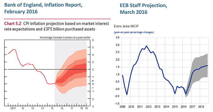
Work continues on enhancing our forecasting models because forecasts of inflation are particularly important for monetary policymaking. The fact that it takes considerable time for policy actions to be transmitted through all parts of the economy requires monetary policymakers to be forward looking. Central bankers in the U.S., U.K., and Euro zone are projecting that inflation will rise gradually toward their respective inflation targets over the next couple of years. We should keep in mind that the confidence bands around these forecasts are fairly wide, reflecting model uncertainty, the fact that the economy is constantly being buffeted by shocks, and that the data can be revised over time.¹⁴

Figure 11 illustrates the confidence intervals around forecasts of the Bank of England and ECB staff. In the Bank of England’s projection, the middle band is a 70 percent confidence interval; for the ECB staff forecast it’s a 57.5 percent confidence band – in both cases the width one year out is a little over ±1 percentage point.

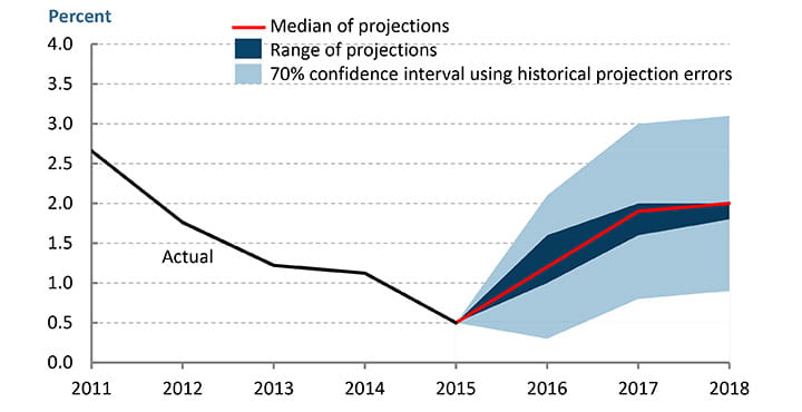
Unlike these central banks, in the U.S., the FOMC does not publish a consensus forecast or a staff forecast. Instead, four times a year, the FOMC summarizes the individual projections of each Committee participant. The median projection of headline PCE inflation published in March indicates that inflation is projected to rise from 0.5 percent in 2015 to 1.2 percent this year and about 2 percent in 2017 and 2018. The FOMC does not produce error bands around these projections, although this is being discussed.¹⁵ The Committee does publish a summary table of the average historical errors of projections from 1996 through 2015 made by various private and government forecasters. For inflation, these errors are around ?1 percentage point one or two years out. We can apply these errors to the median FOMC projection to get an approximate, symmetric 70 percent confidence interval. As seen in Figure 12, although the dispersion across FOMC participants often gets some attention, it is actually quite narrow compared with the confidence bands around forecasts of inflation.

The precision of the forecasts, or lack thereof, needs to be kept in mind when setting monetary policy. We must be forward looking, which means we must rely on models to forecast inflation, but there is no one model that forecasts with much accuracy. The best we can do in this situation is to recognize that there is uncertainty around our forecasts. I am in favor of the FOMC providing some type of error band around its projections. Not only will it help the public understand some of the risks around our forecast, but it will also be a helpful reminder to policymakers that we constantly live with uncertainty. This shouldn’t paralyze us. Instead we should cope with it by looking at the outcomes from multiple models and alternative simulations, using techniques like model averaging, and by continually evaluating the forecasts from the models against incoming data. The FOMC has been expanding the models it routinely examines as a part of the policymaking process — these include the Board of Governors staff’s large-scale FRB/US model and two smaller-scale DSGE models called EDO and SIGMA, as well as various models maintained and utilized at the Federal Reserve Banks. Researchers are now building model archives to aid in the systematic comparison of empirical results and policy implications across a large set of economic models as an aid to policy analysis. One such archive, The Macroeconomic Model Data Base (MMB), headed by Volker Wieland of Goethe University Frankfurt, currently includes 61 models.¹⁶ Given the state of our knowledge, this seems to be a promising approach to ensuring that policy actions are robust across the span of plausible models of economic dynamics and economic circumstances.

Of course, in addition to model averaging, it is also important for central bank and academic researchers to continue to push the envelope of our knowledge. Let me finish by discussing research on inflation expectations, an area that I view as critical to advancing our understanding of inflation dynamics, measurement, and forecasting.

Inflation Expectations Research

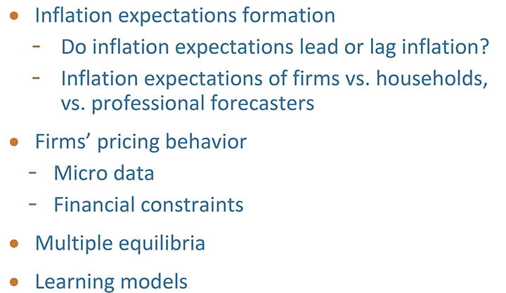
Despite the central role inflation expectations play in our theories of inflation dynamics and monetary policy transmission, there is still much we don’t know about how such expectations are formed or even whose expectations matter for forecasting inflation and setting monetary policy. It took many years to bring inflation expectations down, so keeping inflation expectations anchored at a central bank’s target is a high priority. If inflation runs below or above the targeted inflation rate for some period of time, will it cause longer-term inflation expectations to become unanchored and the public to lose confidence in the central bank? Does it matter how far inflation is from target, or how long it’s been away from the target to trigger such a response? Without a better understanding of how people form their expectations about inflation, it is difficult to answer these questions or to have a good sense of what might cause inflation expectations to become unanchored from the central bank’s target.

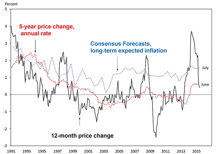
To see that this is not straightforward, one can look at the experience in Japan. As shown in Figure 13, in Japan, after a long period of being stuck near zero, actual inflation ran below zero from 2009 through mid-2013. Even so, measures of inflation expectations were relatively stable between 1.5 and 2 percent, well above actual inflation for a number of years.¹⁷ This presents a conundrum because the theory suggests that changes in inflation expectations should lead changes in underlying inflation.

Inflation expectations may also be an important piece of the puzzle explaining the missing disinflation in the 2009-2011 period (Figure 14). Although the theory is based on firms’ pricing behavior, in the U.S. we don’t have consistent measures of firms’ inflation expectations. Olivier Coibion and Yuriy Gorodnichenko (2015) find that there is a tighter link between the inflation prediction from an estimated Phillips curve and actual inflation when inflation expectations are measured by household expectations than when they are measured by the expectations of professional forecasters.¹⁸ The authors are conducting a survey of firms’ inflation expectations in New Zealand and are already getting some interesting results that suggest that firms’ inflation expectations behave more like the inflation expectations of households than of professional forecasters. In particular, the inflation expectations of firms, like those of households, are considerably higher than those of professional forecasters, and the dispersion across firms is similar to that for households and much wider than that observed across professional forecasters. Firm and household inflation expectations both rose significantly starting in 2009, reflecting the rise in oil prices. Coibion and Gorodnichenko suggest that the fact that disinflationary pressures were absent across countries during the 2009-2011 period lends some support to the idea that a common factor like oil prices, which rose over the period, may have been at work.

A better understanding of firms’ expectations about future inflation may bring us better insight into how firms set prices and may help reconcile some discrepancies between our models and real-world pricing behavior. For example, based on the data on individual prices that are used to construct aggregate price indices like the CPI, Mark Bils and Peter Klenow find that firms appear to change prices more frequently than predicted by standard models that have been calibrated to match various features of the macroeconomic business cycle.¹⁹ This is a troubling finding in that it suggests a disconnect between the micro data and the New Keynesian macro models that are often used to inform monetary policy analysis.

Simon Gilchrist and Egon Zakrajsek are investigating the effect of financial constraints on firms’ pricing behavior. They find that product price inflation varies depending on the ease with which firms can access external finance. Firms with such access can compensate for reduced demand for their products by cutting prices, whereas firms that cannot get such funding need to raise prices to keep revenue from falling too much. Thus, in the wake of a downturn in demand that is accompanied by financial shocks that reduce firms’ access to credit and liquidity, we’d expect to see a drop in output and an increase in markups and, therefore, inflation.²⁰ This is another factor that helps resolve the disinflation puzzle in the aftermath of the Great Recession. These types of results point to the need to further develop DSGE models that seriously incorporate financial markets and the possibility of financial stress, borrower defaults, and financial institution failures. These models need to be fairly complex. By their nature, financial crises involve nonlinearities, potentially multiple equilibria, and financial frictions that limit arbitrage. But there could be a high payoff in terms of furthering our knowledge of inflation dynamics.

Borağan Aruoba and Frank Schorfheide incorporate nonlinearities into a DSGE model so that they can analyze inflation dynamics at and during exit from the zero lower bound on interest rates.²¹ This model has multiple equilibria and the authors examine the two steady states — one in which inflation is at its target and the other in which the nominal interest rate is zero and inflation is negative. Thus, inflation expectations would reflect the public’s expectations about the average inflation rate in each regime as well as their expectations about the probability of switching regimes. Welfare is considerably lower in the deflationary steady state than in the targeted-inflation steady state.

In a world with multiple equilibria, as in this model, one can think of a central bank’s monetary policy as choosing one of the equilibrium paths, which can have very different welfare implications. In the model, the economy can hit the zero lower bound either because of an adverse transitory shock or series of shocks within the targeted-inflation regime, or because the economy has switched to the deflationary regime. Since inflation and interest rates can be low in either regime, knowing which regime the economy is actually in is difficult. This presents a challenge to the central bank, since the optimal monetary policy in each regime differs. Based on their analysis of the inflation and interest rate experiences in the U.S., Euro area, and Japan, the authors suggest that Japan switched into the deflation regime, while it is unlikely that the Euro area did, and the U.S. case is more ambiguous.²²

This type of model can help inform our thinking about the level of the central bank’s inflation target. Our recent experience of the Great Recession has led some economists to suggest that central banks should be targeting a higher inflation rate in normal economic times so that when the economy is hit by sizable shocks there will be more room for conventional expansionary monetary policy.²³ Aruoba and Schorfheide use their model to analyze how output, inflation, and interest rates would have evolved under two different scenarios: first, if the U.S. had picked an inflation target of 4 percent in 1984, and second, if the U.S. were to shift to a 4 percent inflation target now. In the first scenario, after 2009 interest rates do not reach zero, inflation returns quickly to the 4 percent target, output recovers more quickly than under the baseline lower-inflation-target regime, and consumption is higher. However, the authors conclude that the overall benefits of the policy are not clear because there may be costs to adjusting prices to the higher inflation target as well as higher costs of holding cash and other liquid assets at a higher inflation rate. In addition, the benefits depend on the probability of hitting the zero lower bound in the first place.

In the second scenario, the deflation risk is reduced but there is little change in the trajectory of output; thus, there is little real benefit to making such a change. Moreover, other factors that are not modeled suggest that changing the inflation target would be ineffectual and even counterproductive. To the extent that it takes time for the central bank to earn credibility for its inflation target and time for household and business expectations to become anchored at the target, changing the target would have little effect in the short run and be detrimental in the longer run if it undercut credibility and unanchored expectations.

The multiple equilibrium nature of nonlinear DSGE models, like the one built by Aruoba and Schorfheide, suggests that one potentially fruitful area of research is to marry the literature on learning in macroeconomics with the emerging empirical literature on how agents form their expectations. Do people form their expectations based on their own price experience? Do they listen to experts or form expectations based on past inflation rates? Do they have their own theories about what determines future inflation? The concept of rational expectations — that agents’ expectations are consistent with the economic model — was a major advance in macroeconomic theory and is the benchmark assumption in all modern macroeconomic models. Yet it is a strong assumption in that it requires all agents to know the model and its parameters and to know that other agents are rational as well. A literature developed over the past two decades has incorporated various models of learning into macroeconomic models.²⁴ Some of the research finds that expectations eventually converge to rational expectations, but the economic dynamics in such models can differ from those in the benchmark rational expectations model. In addition to exploring the implications of different models of learning — e.g., recursive learning or Bayesian learning — some economists are taking the models to the laboratory to conduct experiments to investigate economic dynamics.²⁵

The learning literature gives us a way to study how the economy might shift from one equilibrium to another.²⁶ Depending on how learning is modeled, such a shift might be gradual or it could be more abrupt, which has implications for economic stability and appropriate policy. Learning models help put some structure on the notion of “anchored” inflation expectations. They potentially point us to factors that might affect the degree to which inflation expectations are anchored to the central bank’s inflation target as well as the role central bank communications and credibility play in individuals’ formation of inflation expectations.

Conclusion

In my remarks today, I have pointed out several open questions about inflation. But rather than being discouraged by what we still don’t know, I am encouraged by the promising avenues being pursued to advance our knowledge about inflation dynamics and inflation expectations. I urge researchers to continue this pursuit because price stability is clearly a goal worth pursuing and good policymaking is dependent on the research that informs it.

Figure 1. Headline inflation

Source: U.S. Bureau of Economic Analysis, ECB, Eurostat via Haver Analytics
Monthly data: Last obs. March 2016
Download charts

Figure 2. Core inflation

Source: U.S. Bureau of Economic Analysis, ECB, Eurostat via Haver Analytics
Monthly data: Last obs. March 2016
Download charts

Figure 3. Other measures of underlying inflation in the U.S.

Source: Federal Reserve Bank of Cleveland and Federal Reserve Bank of Dallas via Haver Analytics
Monthly data: Last obs. March 2016
Download charts

Figure 4. Trend inflation estimates

Source: Federal Reserve Bank of Cleveland
Quarterly data: Last obs. 2015Q4
Download charts

Figure 5. Longer‐term inflation expectations: Surveys of professional forecasters

Source: Federal Reserve Bank of Philadelphia via Haver Analytics, ECB, Bank of England
Quarterly data: Last obs. 2016Q1
Download charts

Figure 6. Longer‐term inflation expectations: Surveys of households

Source: University of Michigan, Bank of England/GfK
Monthly data for U.S.: Last obs. March 2016
Quarterly data for U.K.: Last obs. 2016Q1
Download charts

Figure 7. Five‐year, five‐year forward inflation compensation based on swaps

Source: Bloomberg
Monthly data: Last obs. March 2016
Download charts

Figure 8. Ten‐year inflation risk premia

Source: FRB Cleveland and FRB San Francisco
Monthly data for FRB Cleveland: Last obs. April 2016
Daily data for FRB San Francisco: Last obs. April 7, 2016
Download charts

Figure 9. Five‐year, five‐year forward inflation expectations

Source: FRB Cleveland and FRB San Francisco
Monthly data for FRB Cleveland: Last obs. April 2016
Daily data for FRB San Francisco: Last obs. April 19, 2016
Download charts

Figure 10. The Phillips curve models

Download charts

Figure 11. Confidence intervals around inflation forecasts

Download charts

Figure 12. FOMC’s Summary of Economic Projections: PCE Inflation

Source: FOMC Summary of Economic Projections, March 2016
Download charts

Figure 13. Actual and expected inflation in Japan

Note: The data for the 5-year price change and for the 12-month price change are monthly; the Consensus Forecasts data, which are plotted starting in April 1991, are semiannual through April 2014 and quarterly thereafter. Source: Ministry of Internal Affairs and Communications (Japan); Consensus Economics (London); Haver Analytics.
Source: Janet L. Yellen, “Inflation Dynamics and Monetary Policy,” The Philip Gamble Memorial Lecture, University of Massachusetts, Amherst, MA, September 24, 2015
Download charts

Figure 14. Research on inflation expectations

Download charts

References

- Aruoba, Borağan, Luigi Bocola, and Frank Schorfheide, “Assessing DSGE Model Nonlinearities,” National Bureau of Economic Research Working Paper 19693, 2013.
- Aruoba, Borağan, and Frank Schorfheide, “Inflation During and After the Zero Lower Bound,” Federal Reserve Bank of Kansas City Economic Policy Symposium, Jackson Hole, WY, August 2015.
- Assenza, Tiziana, Peter Heemeijer, Cars Hommes, and Domenico Massaro, “Individual Expectations and Aggregate Macro Behavior,” Tinbergen Institute Discussion Paper 13-016/II, January 5, 2013.
- Bank of England, Inflation Report, February 2016.
- Bernanke, Ben S., “The Benefits of Price Stability,” Center for Economic Policy Studies, Princeton University, Princeton, New Jersey, February 24, 2006.
- Bernanke, Ben S., “Inflation Expectations and Inflation Forecasting,” remarks at the Monetary Economics Workshop of the National Bureau of Economic Research Summer Institute, Cambridge, MA, July 10, 2007.
- Bils, Mark, and Peter J. Klenow, “Some Evidence on the Importance of Sticky Prices,” Journal of Political Economy 112, 2004, pp. 947-985.
- Blanchard, Olivier, Giovanni Dell’Ariccia, and Paolo Mauro, “Rethinking Macroeconomic Policy,” Journal of Money, Credit, and Banking 42, 2010, pp. 119-215.
- Clark, Todd, and Christian Garciga, “Recent Inflation Trends,” Federal Reserve Bank of Cleveland Economic Trends, January 14, 2016.
- Cogley, Timothy, Giorgio E. Primiceri, and Thomas J. Sargent, “Inflation-Gap Persistence in the US,” American Economic Journal: Macroeconomics 2, 2010, pp. 43-69.
- Coibion, Olivier, and Yuriy Gorodnichenko, “Is the Phillips Curve Alive and Well after All? Inflation Expectations and the Missing Disinflation,” American Economic Journal: Macroeconomics 7, January 2015, pp. 197-232.
- Constâncio, Vítor, “Understanding Inflation Dynamics and Monetary Policy,” remarks at the Federal Reserve Bank of Kansas City Economic Policy Symposium, Jackson Hole, WY, August 29, 2015.
- European Central Bank, ECB Staff Macroeconomic Projections for the Euro Area, March 2016.
- Evans, George W., and Seppo Honkapohja, “Learning and Macroeconomics,” The Annual Review of Economics 1, 2009, pp. 421-449.
- Faust, Jon, and Jonathan H. Wright, “Forecasting Inflation,” in Handbook of Economic Forecasting, Graham Elliott and Allan Timmermann, eds., Amsterdam: Elsevier Press, vol. 2A, 2013, pp. 2-56.
- Fischer, Stanley, “U.S. Inflation Developments,” remarks at the Federal Reserve Bank of Kansas City Economic Policy Symposium, Jackson Hole, WY, August 29, 2015.
- Fratianni, Michele, and Jürgen von Hagen, “The Konstanz Seminar on Monetary Theory and Policy at Thirty,” May 2001.
- Gilchrist, Simon, Raphael Schoenle, Jae W. Sim, and Egon Zakrajsek, “Inflation Dynamics During the Financial Crisis,” Board of Governors of the Federal Reserve System, Finance and Economics Discussion Series 2015-012, March 3, 2015.
- Larkin, John, “Box A: Oil Prices and Inflation Expectations: An Investigation Into the Contribution of Global Demand and Oil Supply Shocks to Euro Area Inflation Expectations,” in Central Bank of Ireland, Quarterly Bulletin 02, April 2016, pp. 47-48.
- Mester, Loretta J., “Inflation and Monetary Policy: Six Research Questions,” speech before the 2014 Inflation Conference hosted by the Federal Reserve Bank of Cleveland, May 29, 2014.
- Minutes of the FOMC Meeting of January 26-27, 2016.
- Nakamura, Emi, and Jón Steinsson, “Five Facts about Prices: A Reevaluation of Menu Cost Models,” Quarterly Journal of Economics, November 2008, pp. 1415-1464.
- Orphanides, Athanasios, “Monetary Policy Rules and the Great Inflation,” American Economic Review 92, 2002, pp. 115–120.
- Orphanides, Athanasios, “Inflation Dynamics: Lessons From Past Debates for Current Policy,” remarks at the Federal Reserve Bank of Kansas City Economic Policy Symposium, Jackson Hole, WY, August 29, 2015.
- Orphanides, Athanasios, and Simon Van Norden, “The Reliability of Inflation Forecasts Based on Output Gap Estimates in Real Time,” Journal of Money, Credit, and Banking, 37, 2005, pp. 583-601.
- Orphanides, Athanasios, and John C. Williams, “Learning, Expectations Formation, and the Pitfalls of Optimal Control Monetary Policy,” Journal of Monetary Economics 55, 2008, S80-S96.
- Plosser, Charles I., “Strengthening Our Monetary Policy Framework,” 20th Annual Hyman P. Minsky Conference, New York, NY, April 14, 2011.
- Rosengren, Eric S., “Changing Economic Relationships: Implications for Monetary Policy and Simple Monetary Policy Rules,” Chatham House, London, England, April 16, 2015.
- Sill, Keith, “Inflation Dynamics and the New Keynesian Phillips Curve,” Federal Reserve Bank of Philadelphia Business Review, Q1 2011, pp. 17-25.
- The Macroeconomic Model Data Base (MMB) web page.
- Trehan, Bharat, and Maura Lynch, “Consumer Inflation Views in Three Countries,” Economic Letter, Federal Reserve Bank of San Francisco, November 2013.
- Wieland, Volker, Tobias Cwik, Gernot J. Müller, Sebastian Schmidt, and Maik Wolters, “A New Comparative Approach to Macroeconomic Modeling and Policy Analysis,” Journal of Economic Behavior and Organization 83, 2012, pp. 523-541.
- Yellen, Janet L., “Inflation Dynamics and Monetary Policy,” The Philip Gamble Memorial Lecture, University of Massachusetts, Amherst, MA, September 24, 2015.