

- Share
A Growth-Augmented Phillips Curve
Empirical studies find that the link between inflation and economic slack has weakened in recent decades, a development that could hamper monetary policymakers as they aim to achieve their inflation objective. We show that while the role of economic slack has diminished, economic growth has become a significant driver of inflation dynamics, indicating that the link between inflation and economic activity remains but the relevant gauge of activity has changed. The new evidence suggests that the COVID-19-related recession could induce substantial disinflationary pressure.

The views authors express in Economic Commentary are theirs and not necessarily those of the Federal Reserve Bank of Cleveland or the Board of Governors of the Federal Reserve System. The series editor is Tasia Hane. This paper and its data are subject to revision; please visit clevelandfed.org for updates.
Empirical studies show that whether the economy’s productive resources are used to full capacity or economic conditions are slack has become less important for inflation dynamics since around the mid-1980s.1 The relationship between inflation and economic slack, commonly measured as the gap between either unemployment and its potential level or output and its potential level, is captured by the Phillips curve. The diminished role of economic slack became apparent during the recession of 2007–2009, when inflation remained surprisingly stable in the face of an elevated unemployment rate that prompted Phillips-curve-based predictions of deflation. The “missing deflation” during the recession was followed by “missing reflation” in the subsequent expansion, as unemployment fell to historic lows but inflation remained subdued.
A weakened link between inflation and economic activity poses a challenge for monetary policymakers. Contemporary models of monetary policy rely on the Phillips curve for the transmission of monetary policy to inflation. A diminished influence of economic slack on inflation—a flatter Phillips curve—indicates that policymakers face a costlier trade-off between economic activity and inflation, because a desired increase or decrease in inflation would require, respectively, a greater increase or decrease in economic activity.2
But does the flatter Phillips curve really imply that the relationship between inflation and economic activity has weakened? In this article, we revisit the relationship by focusing on the role of economic growth for inflation dynamics. We present empirical evidence from an estimated Phillips curve model that shows economic growth has become a significant driver of inflation dynamics since the previous recession. The evidence indicates that inflation continues to be influenced by economic activity, but growth has replaced slack as the relevant gauge of activity. Based on a medium-term forecast for economic growth that incorporates a severe COVID-19-related recession, the model predicts a period of subdued inflation.
A Phillips Curve with Output Growth
While monetary policymakers have traditionally focused on the role of economic slack for inflation dynamics, theory suggests there could be a role for economic growth as well. Theoretical Phillips curves are derived from the price-setting decisions of firms that face costly price adjustment, but the precise specification of the Phillips curve also depends on the behavior of households in the theoretical model economy. A model wherein habit formation leads households to care about increases in consumption, rather than absolute consumption levels, implies that the Phillips curve includes economic growth as a determinant of inflation.3 The assumption of habit formation is commonly used in finance and business cycle analyses to address various issues not necessarily related to inflation. The benchmark theoretical Phillips curve, the so-called New Keynesian Phillips curve (NKPC), relates inflation to expectations of future inflation and to an output gap that captures economic slack (see, e.g., Woodford, 2003). Introducing the assumption of habit formation allows us to extend the benchmark theoretical Phillips curve by adding output growth as an additional determinant of inflation. The NKPC can then be written mathematically as
(1) πt = βπet+1 + αy yt + αg gt + ut
where πt denotes inflation at time t, yt denotes the output gap, gt is output growth, and the coefficients αy and αg represent the sensitivity of inflation to the output gap and to output growth, respectively. The variable πet+1 denotes expected inflation in the next period, and ut is an error term added for the empirical analysis.4 Using the NKPC of equation (1), we empirically investigate the importance of output growth for inflation dynamics.
Our empirical analysis builds on that of Ball and Mazumder (2011) by augmenting their empirical Phillips curve model, which relates inflation to inflation expectations and economic slack, with a term for economic growth motivated by the NKPC in equation (1).5 We adopt two measures of inflation expectations, one backward-looking and one forward-looking, which between them encompass a range of possible views on expectations formation. The backward-looking measure assumes, as in Ball and Mazumder (2011), that expectations are determined by the average inflation rate of the past four quarters, implying that shocks to inflation have persistent effects. The forward-looking measure is a survey-based measure of long-term inflation expectations and implies that shocks to inflation may have only transitory effects if inflation expectations remain anchored.6 We estimate the model on quarterly data from the first quarter of 1960 to the fourth quarter of 2019, extending the data sample of Ball and Mazumder (2011) by nine years.
Stronger Association between Inflation and Output Growth
Our estimated Phillips curve model indicates that the association of inflation with output growth has strengthened since the 2007–2009 recession, while the association with the output gap has remained weak. Table 1 presents regression estimates of the Phillips curve coefficients, using lagged inflation to proxy for inflation expectations in panel A and long-term inflation expectations in panel B.7
Table 1. Results of Phillips Curve Regressions for Different Sample Periods
| Sample period | αy | αg | Adjusted R2 |
|---|---|---|---|
| Panel A. Lagged inflation | |||
| 1960–1984 | 0.212*** | −0.217 | 0.818 |
| (0.047) | (0.149) | ||
| 1985–2019 | 0.002 | 0.245* | 0.713 |
| (0.034) | (0.133) | ||
| 1985–2007 | 0.058 | 0.089 | 0.717 |
| (0.036) | (0.110) | ||
| 2008–2019 | −0.041 | 0.460** | 0.230 |
| (0.050) | (0.185) | ||
| 2008–2019 | … | 0.423*** | 0.270 |
| (0.164) | |||
| Panel B. Inflation expectations | |||
| 1960–1984 | 0.197*** | −0.583*** | 0.637 |
| (0.065) | (0.222) | ||
| 1985–2019 | 0.065* | −0.030 | 0.711 |
| (0.035) | (0.143) | ||
| 1985–2007 | 0.099* | −0.285*** | 0.704 |
| (0.055) | (0.104) | ||
| 2008–2019 | 0.059 | 0.329** | 0.147 |
| (0.037) | (0.141) | ||
| 2008–2019 | … | 0.381*** | 0.149 |
| (0.142) | |||
Notes: The table reports OLS regression results with Newey-West standard errors in parentheses. The ellipsis (…) indicates that the parameter estimate is not available. The ***, **, and * denote statistical significance at the 1 percent, 5 percent, and 10 percent levels, respectively.
Sources: Bureau of Labor Statistics, Bureau of Economic Analysis, Congressional Budget Office, Federal Reserve Board of Governors, Haver Analytics, and authors’ calculations.
We discuss first the empirical results for the specification with lagged inflation. Previous research shows a decline in the sensitivity of inflation to economic slack around the mid-1980s. Thus, the first two lines of panel A break the sample into the period from the first quarter of 1960 to the fourth quarter of 1984 and the post-1984 period from the first quarter of 1985 to the fourth quarter of 2019. The estimated coefficient for the output gap declined from 0.212 to essentially zero between these periods, reflecting the flattening of the Phillips curve noted in previous research. The estimated coefficient for output growth was negative in the first period, which includes the stagflation of the 1970s, and turned positive (0.245) after the mid-1980s.8
The positive estimate for the post-1984 period reflects a noticeable strengthening of the association between inflation and output growth around the start of the previous recession. Indeed, estimation results for a version of the Phillips curve with time-varying coefficients, presented in the online appendix, show an increase in the coefficient for output growth around the onset of the last recession. Based on the break indicated by the time-varying coefficient, the next two lines of the table split the post-1984 sample in the first quarter of 2008. This reveals that the estimated coefficient for output growth has become more economically significant, rising from 0.089 to 0.460, and statistically significant since 2008.9 In contrast, the coefficient for the output gap has remained near zero since the last recession, which is the period characterized by “missing deflation” and “missing reflation.” Because the coefficient for the output gap was not significantly different from zero in the most recent time period, the last line of panel A drops the output gap from the regression.
Using the survey-based measure of long-term inflation expectations instead of lagged inflation to proxy for inflation expectations, panel B shows similar patterns across time periods. Specifically, the estimation indicates that the Phillips curve flattened in the post-1984 period, and the association between inflation and output growth has strengthened since 2008.10 The break in 2008 is even starker in panel B than in panel A, as the coefficient for output growth switches sign, increasing from −0.285 to 0.329. Overall, the results reported in table 1 indicate that economic growth has become a significant driver of inflation dynamics, suggesting that fluctuations in growth could affect inflation going forward.11
Implications of the Recession for Inflation
The US economy experienced a severe recession caused by the COVID-19 pandemic and the social-distancing actions taken to stem the spread of the coronavirus. Based on the existing evidence that the Phillips curve has flattened, one might conclude that the decline in aggregate demand will likely leave a limited imprint on inflation. In contrast, the evidence in table 1 suggests that inflation could be affected substantially by the contraction in real GDP. To get a sense of the possible effects, we forecast inflation by feeding a forecast of real GDP growth into our Phillips curve regressions estimated on the data from 2008 to 2019, using the specification with lagged inflation and that with long-term inflation expectations.12
Figure 1 displays the four-quarter core PCE inflation rate and its forecast from the estimated Phillips curve regressions in panel A, along with real GDP growth and the Blue Chip consensus forecast of real GDP growth in panel B. The Blue Chip survey was conducted in May 2020 and provides a forecast from the second quarter of 2020 to the fourth quarter of 2021. Survey respondents expected real GDP growth to turn sharply negative in the first half of 2020, followed by strong positive growth in the second half of the year as economic activity was expected to return to a more normal pace.13
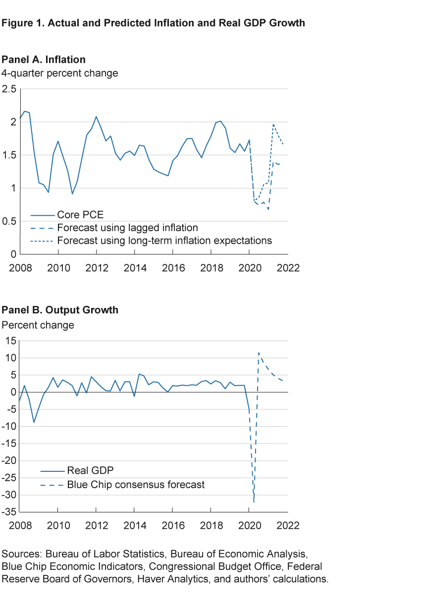
Based on the projected path for real GDP growth, the estimated Phillips curve with lagged inflation predicts persistent weakness in inflation. The recession leads core inflation to decelerate until it reaches 0.7 percent in the first quarter of 2021, despite upward momentum from rising core inflation in 2019. Core inflation picks up somewhat in the remaining three quarters of 2021 but, at 1.4 percent, remains below the Federal Reserve’s inflation target of 2 percent. The prolonged weakness in inflation in 2021, when the Blue Chip forecast calls for strong positive growth, reflects the persistent effects of lagged inflation in the estimated Phillips curve model.
The inflation forecast is more benign if inflation expectations remain anchored. For the inflation forecast of the estimated Phillips curve with long-term inflation expectations, we assume that expectations remain anchored at 1.9 percent—their observed level in the second quarter of 2020—throughout the forecast horizon. The anchored expectations prevent a persistent deceleration of inflation. Instead, the forecast reaches a low of 0.9 percent in the second quarter of 2020, coinciding with the trough in real GDP growth, before gradually rising to around 1.8 percent in the last three quarters of 2021.
Because the two specifications of the Phillips curve encompass a range of views on inflation expectations, from the purely backward-looking to the purely forward-looking, we view the corresponding inflation forecasts as likewise encompassing a range of plausible forecasts. In the more benign scenario, inflation expectations remain anchored, and inflation dips only temporarily. In the more damaging scenario, inflation expectations become unanchored by low inflation readings, leading to a more protracted period of low inflation. A few caveats with these forecasts are worth pointing out. First, the forecast for real GDP growth, like any forecast, is surrounded by uncertainty, which is especially large during recessions (Bloom, 2014). The Phillips curve model then transmits such uncertainty to the inflation forecast. Second, the behavior of macroeconomic aggregates, and thus their relationships, could differ in the current recession from those observed in previous post-World War II recessions. This is because the COVID-19 pandemic and related mandatory and voluntary social-distancing actions likely affect consumers’ and firms’ economic decisions. Those decisions are also influenced by the unprecedented fiscal and monetary policy responses to the recession. Finally, the health pandemic even affects the collection and quality of official statistics, which could affect statistical inferences about the Phillips curve in the future.14
Conclusion
Our analysis confirms the findings of previous research that the link between inflation and economic slack has weakened since around the mid-1980s and presents new evidence that an economically and statistically significant association between inflation and economic growth has emerged since the last recession. The relationship between inflation and economic growth is a reassuring finding for monetary policymakers because it implies that the link between inflation and real activity, on which policymakers rely for the transmission of monetary policy to inflation, has not vanished after all but has merely taken on a different form. However, in the medium term, the relationship implies that the COVID-19-related recession could induce substantial disinflationary pressure that may prove to be persistent.
Footnotes
- See, e.g., Benati (2007), Ball and Mazumder (2011), Matheson and Stavrev (2013), and Del Negro et al. (2020). Return to 1
- The research literature has not yet reached consensus about the reasons why the Phillips curve has flattened. Occhino (2019) reviews possible causes of the flattening and analyzes implications of the different causes for monetary policy. Return to 2
- Intuitively, households’ preferences for (quasi-)changes in consumption produce a Phillips curve with output growth because the preferences affect households’ interactions with firms in the labor market and thereby firms’ production costs and price-setting decisions. Return to 3
- In addition to the error term, there are two other differences between the theoretical NKPC and its empirical counterpart. First, whereas inflation expectations in the theoretical NKPC are formed as rational (that is, model-consistent) expectations, the empirical analysis will impose different assumptions for expectations formation. Second, although theoretically the discount factor β takes a value less than but close to one, we will impose the restriction β=1 in the empirical analysis. The error term is sometimes justified theoretically as a cost-push shock. Return to 4
- Orphanides and van Norden (2005) compare inflation forecasts based on the output gap to forecasts based on output growth and find that the latter can outperform the former if the output gap is measured using real-time data. Return to 5
- The measure of inflation used for estimation is the first difference of the log core personal consumption expenditures (PCE) price index, although the results are robust when using the headline PCE price index. The series of long-term inflation expectations is from the Federal Reserve Board of Governors, denoted PTR in the FRB/US documentation. The quarterly series for inflation and inflation expectations are expressed at annualized rates. The output gap is measured as the deviation of log real GDP from log potential real GDP, wherein the series of potential real GDP is from the Congressional Budget Office. Output growth is measured as the first difference of log real GDP. Return to 6
- Following Ball and Mazumder (2011), the regression models are estimated with ordinary least squares (OLS). A test for regressor endogeneity may alleviate the concern that OLS can yield inconsistent estimates if the output gap or output growth is endogenous. We performed a Durbin–Wu–Hausman test using two-stage least squares with the first four lags of the output gap and output growth as instruments. The null hypothesis that the output gap or output growth is exogenous cannot be rejected. Estimation by OLS then has the advantage that it yields more efficient estimators than instrumental variables estimation. As Fuhrer (2017) points out, the survey expectations of inflation are recorded in the middle of quarter t, so they contain information only for quarter t–1 and earlier. Return to 7
- Adding output growth to the Phillips curve regressions with the output gap and either lagged inflation or survey-based inflation expectations improves the model fit noticeably in some sample periods, as judged by the adjusted R-squared. Specifically, the adjusted R-squared increases between 1.1 percentage points and 9.3 percentage points for the sample periods 1960 to 1984 and 2008 to 2019. The adjusted R-squared remains roughly unchanged for the sample periods beginning in 1985. Return to 8
- Why the coefficient for output growth has increased is a question for further research. The theoretical NKPC relates the coefficient to a number of structural parameters, so changes in those parameters would change the coefficient. Moreover, a change in the conduct of monetary policy could alter the estimated coefficient in the empirical Phillips curve. For example, a more forceful response of monetary policy to fluctuations in output growth could dampen such fluctuations relative to the movements in inflation, thereby increasing the estimated elasticity of inflation with respect to output growth. Empirical estimates of the Federal Reserve’s interest rate policy rule indicate that its policy response to output growth has increased and that its policy response to the output gap has declined since the mid-1980s (Coibion and Gorodnichenko, 2011; Hirose, Kurozumi, and Van Zandweghe, 2020). McLeay and Tenreyro (2020) show that the conduct of monetary policy affects the empirical estimate of the slope of the Phillips curve. Return to 9
- One difference between panels A and B is that in the latter the coefficient for the output gap remains significant in the post-1984 period, a finding that is consistent with the regression results using survey-based inflation expectations reported by Ball and Mazumder (2019). Return to 10
- We estimated the same regressions with alternative measures of economic slack and economic growth to assess the robustness of the results. Using the unemployment gap, the short-term unemployment gap defined by Ball and Mazumder (2019), or the unemployment recession gap of Stock and Watson (2010) produces qualitatively similar results as those reported in table 1. The unemployment gap is the deviation of the unemployment rate from the Congressional Budget Office’s NAIRU series; the short-term unemployment gap is the fraction of the labor force unemployed for 26 weeks or fewer minus 0.8516 times the NAIRU; the unemployment recession gap is the difference between the current unemployment rate and the minimum unemployment rate over the current and previous 11 quarters. Likewise, the results were qualitatively similar when replacing real GDP growth with the growth rate of nonfarm payroll employment or of the output gap. Return to 11
- For the forecasts, we use the results obtained with the regressions that omit the output gap, regressions that are reported in the last lines of each panel in table 1. Although observations for core PCE inflation and real GDP growth in the first quarter of 2020 are available at the time of writing, we end the sample for estimation in the fourth quarter of 2019 because it is the last quarter before the COVID-19-related downturn started. Return to 12
- See Wolters Kluwer Legal and Regulatory Solutions US, Blue Chip Economic Indicators, 45(5), May 10, 2020. Return to 13
- Recent news releases for the labor market and the consumer price index discuss the possible effects of the pandemic on official statistics (Bureau of Labor Statistics, “The Employment Situation—April 2020,” May 8, 2020, and Bureau of Labor Statistics, “Consumer Price Index—April 2020,” May 12, 2020). Return to 14
References
- Ball, Laurence, and Sandeep Mazumder. 2011. “Inflation Dynamics and the Great Recession.” Brookings Papers on Economic Activity, 42(1): 337–381. https://doi.org/10.1353/eca.2011.0005.
- Ball, Laurence, and Sandeep Mazumder. 2019. “A Phillips Curve with Anchored Expectations and Short-Term Unemployment.” Journal of Money, Credit, and Banking, 51(1): 111–137.
- Benati, Luca. 2007. “The Time-Varying Phillips Correlation.” Journal of Money, Credit, and Banking, 39(5): 1275–1283.
- Bloom, Nicholas. 2014. “Fluctuations in Uncertainty.” Journal of Economic Perspectives, 28(2): 153–176. https://doi.org/10.1257/jep.28.2.153.
- Coibion, Olivier, and Yuriy Gorodnichenko. 2011. “Monetary Policy, Trend Inflation, and the Great Moderation: An Alternative Interpretation.” American Economic Review, 101(1): 341-370. https://doi.org/10.1257/aer.101.1.341.
- Del Negro, Marco, Michele Lenza, Giorgio E. Primiceri, and Andrea Tambalotti. 2020. “What’s up with the Phillips Curve?” Brookings Papers on Economic Activity, Spring 2020 Edition. https://www.brookings.edu/bpea-articles/whats-up-with-the-phillips-curve/.
- Fuhrer, Jeff. 2017. “Expectations as a Source of Macroeconomic Persistence: Evidence from Survey Expectations in a Dynamic Macro Model,” Journal of Monetary Economics, 86: 22-35. https://doi.org/10.1016/j.jmoneco.2016.12.003.
- Hirose, Yasuo, Takushi Kurozumi, and Willem Van Zandweghe. 2020. “Monetary Policy and Macroeconomic Stability Revisited.” Review of Economic Dynamics, 37: 255–274. https://doi.org/10.1016/j.red.2020.03.001.
- Matheson, Troy, and Emil Stavrev. 2013. “The Great Recession and the Inflation Puzzle.” Economics Letters, 120(3): 468–472. https://doi.org/10.1016/j.econlet.2013.06.001.
- McLeay, Michael, and Silvana Tenreyro. 2020. “Optimal Inflation and the Identification of the Phillips Curve.” In Martin S. Eichenbaum, Erik Hurst, and Jonathan A. Parker (Eds.), NBER Macroeconomics Annual 2019, National Bureau of Economic Research, University of Chicago Press: 199–255. https://doi.org/10.1086/707181.
- Occhino, Filippo. 2019. “The Flattening of the Phillips Curve: Policy Implications Depend on the Cause.” Federal Reserve Bank of Cleveland, Economic Commentary, 2019-11. https://doi.org/10.26509/frbc-ec-201911.
- Orphanides, Athanasios, and Simon van Norden. 2005. “The Reliability of Inflation Forecasts Based on Output Gap Estimates in Real Time.” Journal of Money, Credit and Banking, 37(3): 583–601. https://doi.org/10.1353/mcb.2005.0033.
- Stock, James H., and Mark W. Watson. 2010. “Modeling Inflation after the Crisis.” Proceedings Economic Policy Symposium Jackson Hole, Federal Reserve Bank of Kansas City, 173–220. https://doi.org/10.3386/w16488.
- Woodford, Michael. 2003. Interest and Prices: Foundations of a Theory of Monetary Policy. Princeton University Press.
Suggested Citation
Tauber, Kristen, and Willem Van Zandweghe. 2020. “A Growth-Augmented Phillips Curve.” Federal Reserve Bank of Cleveland, Economic Commentary 2020-16. https://doi.org/10.26509/frbc-ec-202016
This work by Federal Reserve Bank of Cleveland is licensed under Creative Commons Attribution-NonCommercial 4.0 International

