

- Share
The Flattening of the Phillips Curve: Policy Implications Depend on the Cause
According to the historical relationship known as the Phillips curve, strengthening of the economy is commonly associated with increasing inflation. With inflation having only modestly picked up in the past few years as the economy has become more robust, many believe the Phillips curve relationship has weakened, with the curve becoming flatter. I show that the flattening can be due to very different types of structural changes and that knowing the type of change that has occurred is crucial for choosing the appropriate monetary policy.
The views authors express in Economic Commentary are theirs and not necessarily those of the Federal Reserve Bank of Cleveland or the Board of Governors of the Federal Reserve System. The series editor is Tasia Hane. This paper and its data are subject to revision; please visit clevelandfed.org for updates.
The recent behavior of inflation in the United States and some other advanced economies has been the subject of considerable analysis and commentary. Many observers have been surprised that inflation hasn’t risen more than it has in the past few years as the economy has continued to strengthen. According to the historical relationship known as the Phillips curve, strengthening of the economy is commonly associated with increasing inflation. With inflation having only modestly picked up in the past few years as the economy has become more robust, many believe the Phillips curve relationship has weakened. This seemingly reduced sensitivity of inflation to economic conditions is commonly referred to as a flattening of the Phillips curve.
The recent experience that suggests a flattening of the Phillips curve has been corroborated by some research.1 What is less clear is what may have been behind the flattening. The Phillips curve relationship depends on many economic factors, and the flattening may have been caused by a change in any of these factors. One possibility is that the flattening may have been caused by a change in the way monetary policy responds to inflation and economic conditions. Another possibility is that something else fundamental has changed in the economy, for instance the openness of the economy to foreign trade or the way firms set wages and prices.2
What a flatter Phillips curve might mean for the appropriate conduct of monetary policy depends on what has caused the flattening. In this article, I illustrate this point with the help of a modern model of the economy. I first use the model to show that a flatter Phillips curve could be caused by a structural change unrelated to policy or a change in the behavior of monetary policy. I then consider one possible adjustment to the conduct of monetary policy following the flattening and I show that whether the adjustment is appropriate depends on what has caused the flattening.
The Model
To understand possible sources of the flattening of the Phillips curve and its implications for monetary policy, I use a model that is meant to capture the business cycle behavior of the economy. The model—commonly referred to as the New Keynesian model—represents the behavior of households, firms, and monetary policy.3 Households choose work hours and consumption levels to maximize current and expected future utility. Firms produce goods and set prices to maximize profits. The central bank (the Federal Reserve in the United States) sets the short-term interest rate to try to stabilize economic activity and inflation. A key feature of this modern model is that the agents in the model are forward-looking. Expectations of future output, inflation, and interest rates play key roles in determining current economic outcomes.
One important assumption of the model is that firms are slow to adjust prices, an assumption referred to as sticky prices. This assumption is meant to replicate in a stylized way that the prices of goods and services are slow to change in the real world. The model assumes that, in each period, a random fraction of firms, θ, cannot change the prices of the goods they sell. With this assumption, the parameter θ controls how sticky the price level is in the economy: the higher θ, the stickier the price level.
The main macroeconomic variables are output, inflation, and the interest rate. Let yt, πt, and it, denote, respectively, the logarithm of output (or log-output), the inflation rate, and the nominal interest rate. The goal of the model is to characterize the dynamics of these macroeconomic variables given the dynamics of three kinds of macroeconomic shocks that hit the economy (a technology shock, a demand shock, and a monetary policy shock).
The model makes use of a few key concepts. One is known as the steady state. The steady-state value of a variable is the one that will prevail in the long run, after business cycle influences have died out. The model focuses on fluctuations of log-output, inflation, and the interest rate around their steady-state values. In the rest of this article, y will denote the steady-state level of log-output, and ŷt = yt, − y will denote the deviation of log-output from its steady-state level, the output deviation for short (approximately equal to the percent deviation of output from its steady state).
The other key concepts embedded in the model are the natural level of output, ynt, the natural rate of interest, rnt, and the output gap, ỹt . The natural level of output and the natural rate of interest refer, respectively, to the levels of log-output and the real interest rate that would be achieved at each point in time if prices were perfectly flexible, rather than sticky. As shown in Galí 2015, the natural level of output depends on the size of the technology shock, while the natural rate of interest depends on the sizes of both the technology shock and the demand shock. The output gap is the difference between the actual level of log-output and its natural level, i.e., ỹt = yt − ynt, and measures the level of aggregate demand relative to the natural level of output. These three variables (ynt , rnt, and ỹt) cannot be observed in the real world, but they are useful in the model to pin down the dynamics of the three variables of interest (log-output, inflation, and the interest rate).
The behavior of households, firms, and monetary policy is captured by three equations: the dynamic IS equation, which pins down the determinants of aggregate demand, the New Keynesian Phillips curve, which characterizes the dynamics of inflation, and the monetary policy rule, which describes how the central bank sets the interest rate.
The dynamic IS equation, which results from the labor-consumption-saving choices of households, relates the current quarter’s output gap, ỹt, to the output gap expected in the next quarter, Et ỹt+1, the current nominal interest rate, it, the expected inflation rate next quarter, Et πt+1, and the current natural rate of interest, rnt,:
ỹt = − (1/σ) (it−Et πt+1− rnt) + Et ỹt+1.
All other things held constant, the output gap is larger today the larger it is expected to be next quarter. The term (it − Et πt+1− rnt) can be viewed as the gap between the real interest rate, equal to it − Et πt+1, and the natural rate of interest, rnt,. A higher real interest rate tends to lower the output gap because it encourages households to save and discourages households’ consumption and aggregate demand. The extent to which households respond to changes in the real interest rate is controlled by the parameter σ: As σ increases, households become less willing to shift their consumption from today to the future in response to a given increase in the real interest rate.
The New Keynesian Phillips curve, which results from the price-setting behavior of firms, relates the current quarter’s inflation rate, πt, to the inflation rate expected in the next quarter, Et πt+1, and the current output gap, ỹt:
πt= βEt πt+1 + κỹt
According to the equation, a larger output gap is associated with higher inflation because it reflects a level of aggregate demand higher than the natural level of output. The sensitivity of inflation to the output gap, κ, depends on various nonpolicy parameters, including the degree of price stickiness, θ. As θ increases, κ decreases, so the New Keynesian Phillips curve becomes flatter when prices are stickier. Higher expected inflation next quarter is also associated with higher inflation this quarter. The effect of next quarter’s inflation on current inflation depends on the parameter β, which measures how much households value future utility relative to current utility.
Despite the similar name, the New Keynesian Phillips curve is a different type of relationship relative to the Phillips curve described earlier in the introduction. The New Keynesian Phillips curve is a structural relationship that reflects the deep foundations of the model and is not affected by changes in the behavior of monetary policy. The Phillips curve described earlier, however, can be thought of as a simpler statistical model for predicting inflation from past inflation and economic activity. Changes in the behavior of monetary policy or other changes in the structure of the economy do affect this simple statistical relationship, as we will see.
The third and final equation of the model is the monetary policy rule. The equation, commonly known as the Taylor rule, describes how the central bank sets the interest rate, it, in response to inflation, πt, and the deviation of log-output from its long-run steady state,ŷt:
it = ρ + φπ πt + φy ŷt + νt
The central bank raises the interest rate in response to both higher-than-normal inflation and higher-than-normal economic activity. If inflation rises, raising the interest rate has a contractionary effect on economic activity, which in turn applies downward pressure on inflation and helps contain the initial rise in inflation. If economic activity rises, raising the interest rate limits the initial rise in economic activity and its upward pressure on inflation. The parameters φπ and φy control how aggressively the central bank raises the interest rate in response to, respectively, inflation and economic activity. The parameter ρ, equal to ‑log(β), is the steady-state value of the nominal interest rate.4 The term νt is the monetary policy shock and captures changes in policy that cannot be explained by responses to inflation and economic activity.
Making the model operational for the remainder of the analysis requires setting values for the parameters of the model. Most of the parameter values are set to align with those commonly used in research that is based on the model, but a few are simply set to illustrate the main point of this article in a clear way.5 Armed with the model equations and parameters, I assess the Phillips curve by using computer simulations of the model to generate artificial data on log-output and inflation.6 A final detail worth mentioning is that results about the output gap and output deviation are reported in percentage terms, while results about inflation are reported in annualized percentage rates.
A Flatter Phillips Curve Caused by Two Different Changes
The model of the economy just described allows us to assess what might lead to a flattening of the Phillips curve as represented by a simple statistical relationship. To do so, we need to specify that statistical relationship. Reflecting common practice, I use a statistical model relating inflation to past inflation and a measure of output relative to its trend level (for instance, Kuttner and Robinson, 2010, use a quadratic trend).7 The influence of past inflation is captured by the average inflation rate over the previous year, ![]() = (πt−1+ πt−2+ πt−3+ πt−4)/4. The influence of output relative to trend is captured by the deviation of log-output from its steady-state level, ŷt. The statistical Phillips curve takes the form of a regression of the difference between the current quarter’s inflation, πt, and the previous year’s average inflation,
= (πt−1+ πt−2+ πt−3+ πt−4)/4. The influence of output relative to trend is captured by the deviation of log-output from its steady-state level, ŷt. The statistical Phillips curve takes the form of a regression of the difference between the current quarter’s inflation, πt, and the previous year’s average inflation, ![]() , on the output deviation, ŷt, and a constant:
, on the output deviation, ŷt, and a constant:
πt−![]() = c + b ŷt + ut,
= c + b ŷt + ut,
where b is the regression coefficient, c is the constant, and ut is the error term. The regression coefficient, b, is the slope of the Phillips curve. If the slope is positive, inflation tends to rise above its previous-year average level when output is higher than its steady state, and inflation tends to fall when output is lower. If the slope is negative, the opposite relationships tend to hold.
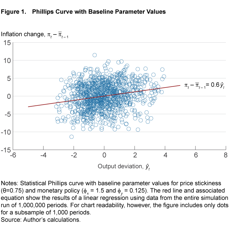
With our baseline parameter values, the model yields a Phillips curve with a positive slope. Figure 1 shows artificial data on the inflation change, πt − ![]() and the output deviation, ŷt, obtained with computer simulations of the model. As indicated by the regression line in figure 1, the estimated regression coefficient b is 0.6, meaning that annualized inflation tends to rise by 0.6 percentage points above its average level in the previous year for each percentage point that output is higher than its steady state (the estimated constant c is very close to zero in all regressions in this article).
and the output deviation, ŷt, obtained with computer simulations of the model. As indicated by the regression line in figure 1, the estimated regression coefficient b is 0.6, meaning that annualized inflation tends to rise by 0.6 percentage points above its average level in the previous year for each percentage point that output is higher than its steady state (the estimated constant c is very close to zero in all regressions in this article).
With that baseline, we’re in a position to assess how changes in either the behavior of monetary policy or other structural parts of the economy could flatten the statistical version of the Phillips curve. We will consider two cases where the Phillips curve flattens for different reasons.
Case 1. First, let’s consider a flattening due to a change in the structure of the economy that is unrelated to monetary policy. Suppose that firms are able to more rapidly adjust their prices in response to current and expected future demand conditions, i.e., prices are less sticky than in the baseline setting of the model. Specifically, the parameter θ, which controls the degree of price stickiness, is lowered from 0.75 in the baseline to 0.56. In this case, captured in figure 2, the statistical version of the Phillips curve becomes close to flat, so inflation changes are nearly unrelated to output deviations. The estimated regression coefficient b is just 0.05, compared to 0.6 in the baseline setting with stickier prices.
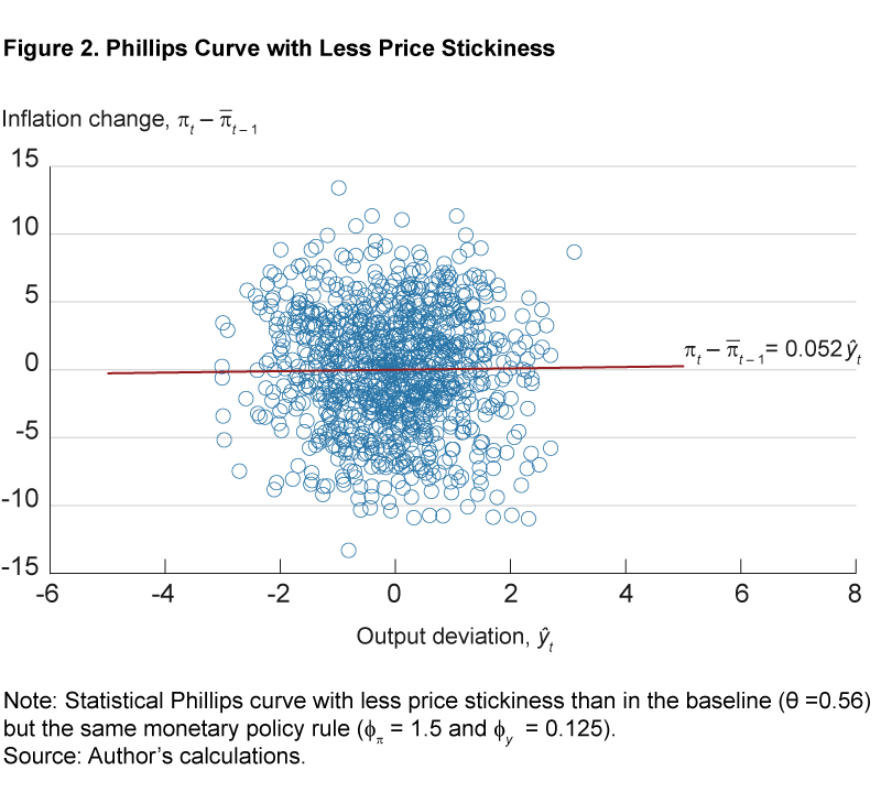
It is interesting that a decrease in price stickiness may cause the statistical Phillips curve (which uses the output deviation) to flatten, even though the New Keynesian Phillips curve (which uses the output gap) becomes steeper. The reason why the statistical Phillips curve flattens in this case is that, when prices become more flexible, the output gap becomes less volatile and less correlated with the output deviation. As a result, inflation, which is directly related to the output gap, also becomes less correlated with the output deviation. As the correlation between inflation and the output deviation decreases, the statistical Phillips curve becomes flatter.8
Case 2. Next, let’s consider a different possible source of a flattening of the statistical Phillips curve, a change in the behavior of monetary policy. Suppose that monetary policy responds more aggressively to economic activity than in the baseline setting of the model. Specifically, the parameter φy, which governs the interest rate response to output deviations, is raised from the baseline value of 0.125 to 0.9. In this case, too, captured in figure 3, the statistical version of the Phillips curve becomes close to flat. The estimated regression coefficient b is again about 0.05, compared to 0.6 in the baseline setting.
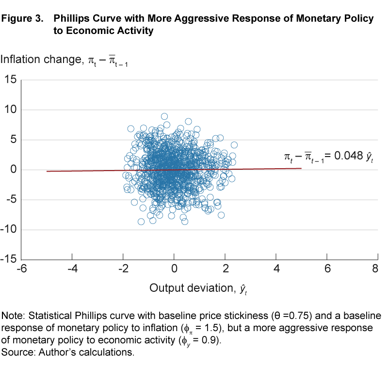
The reason why the statistical Phillips curve flattens in this case is similar to the previous case. As monetary policy responds more aggressively to economic conditions, the output gap becomes less volatile. The correlation between the output gap and the output deviation decreases, leading to a lower correlation between inflation and the output deviation and a flattening of the Phillips curve.9
The slope of the Phillips curve is similar in the two cases, even though the underlying cause of the flattening is different. The general point is that a similar flattening of the Phillips curve can be caused by very different types of changes, a change in the structure of the economy unrelated to policy or a change in the monetary policy rule.
The Welfare Effect of a Policy Adjustment in the Two Cases
Having seen that a flattening of the statistical Phillips curve relationship can have quite different causes, it is natural to ask what the implications for monetary policy might be. The macroeconomic model underlying this article offers a way to address such normative questions. In particular, the household utility—or welfare—embedded in the model can be used to assess alternative policies. More specifically, the model implies that household welfare relates to measures of the volatilities of inflation and the output gap: As the standard deviations of either or both inflation and the output gap increase, household welfare decreases.10 Then, if a policy generates lower standard deviations of both inflation and the output gap, it improves household welfare and is, therefore, preferable.
Following a flattening of the Phillips curve, it seems natural to consider whether monetary policy might improve welfare by reducing the response of the interest rate to economic activity and raising the response to inflation. A flatter Phillips curve could suggest that economic activity has a smaller effect on inflation. If that were the case, on the one hand, the central bank would not need to respond as aggressively to changes in economic activity in order to stabilize inflation. On the other hand, the central bank would need to respond more aggressively to changes in inflation, assuming that the central bank can affect inflation only indirectly by affecting economic activity.
More specifically, let’s consider the effect of adopting a new monetary policy rule where the interest rate stops responding to output deviations (φy=0) and responds slightly more aggressively to inflation (φπ=1.6). Let’s study whether this adjustment to the conduct of monetary policy improves welfare in the two cases described above, namely the case where the flattening is due to less price stickiness (Case 1) and the one where it is due to a more aggressive response of monetary policy to economic activity (Case 2).
In Case 1, the adoption of the new monetary policy rule improves household welfare. The new rule prescribes a less aggressive response to output deviations and a more aggressive response to inflation. While the first effect (a less aggressive response to output deviations) tends to increase the standard deviations of inflation and the output gap, the second effect (a more aggressive response to inflation) tends to decrease them. In this case, the second effect outweighs the first, and the standard deviations of inflation and the output gap decrease (table 1). Household welfare, then, increases.11
| Standard deviation of output gap | Standard deviation of inflation | |
|---|---|---|
| Old policy rule (φπ = 1.5, φy=0.125) |
0.29 | 7.44 |
| New policy rule (φπ = 1.6, φy=0) |
0.25 | 6.47 |
Note: Prices are less sticky than in the baseline (θ=0.56).
Source: Author’s calculations.
In Case 2, however, the adoption of the same monetary policy rule reduces household welfare. As in Case 1, the new rule prescribes a less aggressive response to output deviations and a more aggressive response to inflation. In Case 2, however, the drop in the response to output deviations is much larger than in Case 1 (φy drops by 0.9 in Case 2 compared to 0.125 in Case 1), so the first effect outweighs the second, and the standard deviations of inflation and the output gap increase (table 2). As a result, household welfare decreases.12
| Standard deviation of output gap | Standard deviation of inflation | |
|---|---|---|
| Old policy rule (φπ = 1.5, φy=0.9) |
0.84 | 5.26 |
| New policy rule (φπ = 1.6, φy=0) |
0.96 | 6.07 |
Note: Prices are as sticky as in the baseline (θ=0.75).
Source: Author’s calculations.
In this example, the adoption of the new monetary policy rule has opposite effects on household welfare in the two cases. The takeaway is that whether an adjustment to the conduct of policy is appropriate following the flattening of the Phillips curve depends on the underlying structural change that caused the flattening.
Conclusions
This article has developed examples in which a similar flattening of the Phillips curve is caused by two different types of changes, one a change in the structure of the economy unrelated to policy and the other a change in the behavior of monetary policy itself. The article has shown how the adoption of a new monetary policy rule, unresponsive to output and slightly more aggressive toward inflation, can have opposite effects on household welfare, depending on the cause of the flattening. The general point is that the flattening of the Phillips curve can be due to very different types of structural changes and the type of structural change is crucial for policy implications. When considering whether a change in the conduct of policy is appropriate following a flattening of the Phillips curve, simply knowing that the Phillips curve has flattened is not sufficient, we need to focus on the possible causes.
Footnotes
- See for instance Kuttner and Robinson, 2010; Ball and Mazumder, 2011; Matheson and Stavrev, 2013; and IMF, 2013. Return to 1
- Several studies have suggested that a more responsive monetary policy to inflation and economic conditions, by stabilizing inflation and anchoring inflation expectations, may have been behind the flattening of the Phillips curve, for instance, Haldane and Quah, 1999; Roberts, 2006; Williams, 2006; Mishkin, 2007; Carlstrom, Fuerst, and Paustian, 2009; and McLeay and Tenreyro, 2018. Other studies have pointed to other possible causes including: increased globalization and global competition, which may have made inflation less responsive to domestic demand (IMF, 2006; Borio and Filardo, 2007; Iakova, 2007; and Auer, Borio, and Filardo, 2017), less frequent price adjustments by firms (Kuttner and Robinson, 2010, and Davig, 2016), lower and less volatile inflation, which may have induced less frequent price changes by firms (Ball and Mazumder, 2011), and increased volatility of supply shocks relative to demand shocks (Jacob and van Florenstein Mulder, 2019). [Editor’s note: The final study listed in footnote 2 was not included in the original version; it was added on 9/19/2019.] Return to 2
- The model is the version of the New Keynesian model described in the third chapter of Galí 2015. That chapter explains the model’s derivation and solution as well as the intuition behind it. Return to 3
- The steady-state value of the nominal interest rate is equal to the steady-state value of the real interest rate, because the steady-state value of inflation is equal to zero. In turn, the steady-state value of the real interest rate is equal to ρ, the rate at which households discount future utility relative to the present. Return to 4
- For all the three shocks (technology shock, at, demand shock, zt, and monetary policy shock, νt), the first-order autocorrelations are set equal to 0.9, and the standard deviations equal to 0.5 percent. The other parameters of the model are set as in Galí 2015. In particular, θ = 0.75, implying that on average a firm cannot reset its price for 4 quarters. Also, the monetary policy parameters governing the interest rate response to inflation and output are set equal to, respectively, φπ = 1.5 and φy = 0.125. Return to 5
- The model is simulated for a very large number of periods (1,000,000) so that the numerical results that are reported in this article do not depend in a significant way on the specific realization of the simulation run. Return to 6
- The other common way to specify the statistical Phillips curve is to use a measure of output relative to its potential level, instead of using output relative to its trend level. Since potential output is not observable, authors commonly use the estimates of potential output provided by the Congressional Budget Office (CBO). This approach may be problematic if one wants to investigate whether the Phillips curve has changed over time, because the CBO’s estimates for the period up to 2004 are derived using a Phillips curve that is assumed to be stable over time (Shackleton 2018). Return to 7
- To better understand what is behind the flattening, let’s take a look at the relationship between the output deviation and the output gap. The output deviation, ŷt , can be decomposed into the sum of two components, the output gap, ỹt, and the deviation of natural output from its steady state, (ynt − y). When prices become more flexible, the output gap, ỹt, becomes less volatile. As a result, the ỹt component becomes less important relative to the (ynt − y) component in driving changes in ŷt, so the correlation betweenŷt and ỹt decreases. Since in our example, inflation and ỹt are perfectly positively correlated, the correlation between inflation and ŷt decreases as well, which causes the statistical Phillips curve to flatten. Return to 8
- In addition, ỹt and (ynt − y ) become more negatively correlated, which leads to an even lower correlation between the output gap and the output deviation, and between inflation and the output deviation. Return to 9
- See Galí 2015, Appendix 4.1. Return to 10
- The average quarterly welfare loss relative to the efficient allocation (expressed as the equivalent permanent consumption decline as a percentage of steady-state consumption) decreases from 1.78 percent to 1.35 percent. As the average quarterly welfare loss decreases, household welfare increases. Return to 11
- The average quarterly welfare loss relative to the efficient allocation increases from 3.66 percent to 4.86 percent. As the average quarterly welfare loss increases, household welfare decreases. Return to 12
References
- Auer, Raphael, Claudio Borio, and Andrew Filardo. 2007. “The Globalisation of Inflation: The Growing Importance of Global Value Chains.” Bank for International Settlements Working Paper No. 602.
- Ball, Laurence, and Sandeep Mazumder. 2011. “Inflation Dynamics and the Great Recession.” Brookings Papers on Economic Activity, 42(1): 337–381.
- Borio, Claudio, and Andrew Filardo. 2007. “Globalisation and Inflation: New Cross-Country Evidence on the Global Determinants of Domestic Inflation,” Bank for International Settlements Working Paper No. 227.
- Carlstrom, Charles T., Timothy S. Fuerst, and Matthias Paustian. 2009. “Inflation Persistence, Monetary Policy, and the Great Moderation.” Journal of Money, Credit, and Banking, 41(4), 767–786.
- Davig, Troy. 2016. “Phillips Curve Instability and Optimal Monetary Policy.” Journal of Money, Credit, and Banking, 48(1), 233–246.
- Galí, Jordi. 2015. Monetary Policy, Inflation, and the Business Cycle: An Introduction to the New Keynesian Framework and Its Applications, second edition, Princeton University Press.
- Haldane, Andrew, and Danny Quah. 1999. “UK Phillips Curves and Monetary Policy.” Journal of Monetary Economics, 44(2): 259–278.
- Iakova, Dora M. 2007. “Flattening of the Phillips Curve: Implications for Monetary Policy.” IMF Working Paper, WP/07/76.
- IMF. 2006. “How Has Globalization Affected Inflation?” World Economic Outlook, IMF, Chapter 3.
- IMF. 2013. “The Dog That Didn’t Bark: Has Inflation Been Muzzled or Was It Just Sleeping?” World Economic Outlook, IMF, Chapter 3.
- Jacob, Punnoose, and Thomas van Florenstein Mulder. 2019. “The Flattening of the Phillips Curve: Rounding Up the Suspects.” Reserve Bank of New Zealand Analytical Note Series AN2019/06.
- Kuttner, Ken, and Tim Robinson. 2010. “Understanding the Flattening of the Phillips Curve.” North American Journal of Economics and Finance, 21: 110–125.
- McLeay, Michael, and Silvana Tenreyro. 2018. “Optimal Inflation and the Identification of the Phillips Curve.” CEPR Discussion Paper No. 12981.
- Matheson, Troy, and Emil Stavrev. 2013. “The Great Recession and the Inflation Puzzle.” Economics Letters, 120: 468–472.
- Mishkin, Frederic S. 2007. “Inflation Dynamics.” NBER Working Paper No. 13147.
- Roberts, John M. 2006. “Monetary Policy and Inflation Dynamics.” International Journal of Central Banking, 193–230.
- Shackleton, Robert. 2018. “Estimating and Projecting Potential Output Using CBO’s Forecasting Growth Model.” CBO Working Paper No. 2018–03.
- Williams, John C. 2006. “The Phillips Curve in an Era of Well-Anchored Inflation Expectations.” Unpublished working paper, Federal Reserve Bank of San Francisco.
Suggested Citation
Occhino, Filippo. 2019. “The Flattening of the Phillips Curve: Policy Implications Depend on the Cause.” Federal Reserve Bank of Cleveland, Economic Commentary 2019-11. https://doi.org/10.26509/frbc-ec-201911
This work by Federal Reserve Bank of Cleveland is licensed under Creative Commons Attribution-NonCommercial 4.0 International

