Shocks and the Economic Outlook

During the opening months of 2011, the U.S. economy was beset by a number of shocks. In January and early February, unusually strong and widespread winter storms pummelled the country. These brought construction projects to a halt, left necessary parts and materials stranded in warehouses, and disrupted factory production schedules. Further disruptions followed in the wake of the March 11 Japanese earthquake and tsunami, as U.S industries reliant on components imported from Japan, including automotive parts and semiconductors, had to scale back production.

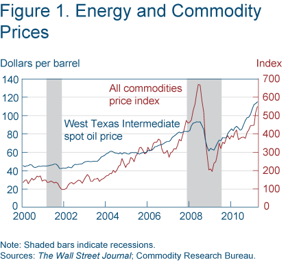
But perhaps the most significant shock has been the political uprisings in the Middle Eastern and North African countries. These tumultuous events drove the price of oil roughly $15 to $20 per barrel higher—a movement that reflects not so much current supply disruptions, but more so the heightened risk to future oil supplies. Sudden spikes in the price of oil occupy a special place in macroeconomic analysis, as really large ones are often followed by slowdowns in economic activity and even recessions. But the run-up in energy prices—along with other industrial commodity prices—has also led to widespread concerns about inflation (figure 1).

 

Economists refer to such events as “supply shocks” in that they disrupt production activities in one way or another. What are the economic consequences of these shocks, and how might they influence the outlook for U.S. economic growth and consumer price inflation? Macroeconomic theory produces clear qualitative descriptions of an economy’s response to supply shocks, but it is less apt at quantifying these effects. In this Commentary, I briefly outline the economic principles that underlie the effects of supply shocks, and then apply a smaller version of a forecasting model in use at the Federal Reserve Bank of Cleveland to help quantify those effects in the current environment.

Output and Inflation Dynamics

To discuss economic dynamics, economists often frame the passage of time in terms of the short, intermediate, and long run. In what follows, the short run is to be understood as one or two quarters after the onset of a temporary shock. It can be thought of as the length of time over which the “impact effect” of the shock is sustained. The intermediate run is the length of time it takes for the shock to play itself out in the economy—typically a period of between two and five years. Beyond the intermediate run, the long run describes the economy after the shock’s effects have been completely played out.

In the long run, the rate at which an economy grows is mainly determined by three factors: the growth rate of the labor force, the rate at which capital equipment and structures are accumulated, and productivity growth. Note that these forces are “real” and not monetary in nature. Long-run inflation, on the other hand, is dominated by monetary considerations and is therefore under the control of the central bank. But in the short and medium run, real and monetary forces jointly influence both growth and inflation.

The course of economic growth and the path of inflation depend to a large extent on the production and pricing behaviors of firms. As a consequence, the modern workhorse theoretical macroeconomic models pay particular attention to incorporating these behaviors.

Like actual businesses, the firms in these models possess some degree of market power or the ability to set a price in excess of production costs. Specifically, the prices they set reflect their marginal cost of production—the real cost of producing an additional unit of output—and a markup over this cost.

Production costs naturally arise from a firm’s purchases of production inputs, including labor services and materials. Consider the example of labor—fundamental to the production of virtually everything. Firms hire workers at market compensation levels. If software engineers are highly sought after and there are not many to be found, then real compensation for these workers will be considerable. The per unit labor cost of a firm naturally depends on the productivity of its employees, too. Relatively productive employees produce more output in a given hour, which spreads out their hourly compensation over more units of output and keeps the real marginal cost of production low.

Although labor is a critically important input, it is not the only one. Production costs also reflect the cost of materials and the ability with which a firm can substitute among materials and between labor and materials more generally. Final goods prices will rise or fall then, when either real unit labor costs or energy and materials prices rise or fall. If we wish to predict real economic activity and inflation, we need a model that includes roles for labor productivity, compensation, commodity prices, and monetary policy, and it needs to be able to disentangle their intertwined roles in output and inflation dynamics.

In principle, a supply shock affects output and prices in the following way. Consider a sudden and unexpected jump in oil prices not unlike the one caused by the Middle Eastern and African political turmoil. Distilled into the primary transportation fossil fuels (such as gasoline, diesel oil, jet fuel) the initial increase in oil prices raises production costs to all who must move goods. The production of various plastics, a ubiquitous intermediate material, depends heavily on crude oil and natural gas. Other industrial chemical inputs derive from crude oil. Clearly, production costs across wide swaths of the economy move higher.

At the firm level, a sudden and unexpected rise in the price of a key material input (such as crude oil) makes it unprofitable to expand output. The rise in marginal cost signals the firm to reduce output and to raise its price. For a variety of reasons though, it is impractical or unwise for firms to continually reset prices in the face of changing cost conditions. Instead, they will sometimes allow their markup to fluctuate to absorb a change in costs. Although not all firms will respond with output reductions and higher prices, some will. So, in the aggregate, we expect to observe slower GDP growth and increases in final goods prices.

A temporary supply shock, though, cannot be the proximate cause of inflation, which by definition is a sustained increase in the rate of growth of the price level. If however, the temporary increase in final goods prices is misperceived to be longer lasting, inflation expectations will move higher—an event that can indeed generate an inflationary episode. In the long run, inappropriately accommodative monetary policy causes inflation to run above a suitable target rate.

A BVAR Forecasting Model

Macroeconomic forecasters have in their toolkit a powerful class of models called Bayesian vector-autoregressive, or BVAR (pronounced BEE-vahr), models that capture the complex and dynamic nature of actual economies. They are flexible and can be expanded to include a number of variables that are relevant to both real activity and inflation. For the present inquiry, that means labor productivity and compensation, commodity prices, and some other relevant variables.

The “Bayesian” part of BVAR means that “extra-sample” beliefs held by the forecaster may be introduced into the forecast along with the degree of confidence that he or she attaches to these beliefs. For BVARs, these so-called “priors” typically represent commonly held views about the long-term properties of macroeconomic time series. In essence, the additional information allows the statistical procedures that quantify the interrelationships to work more efficiently—to make the best use of a limited amount of data. The “vector” part of the name simply means that the models forecast a number of economic concepts at once, not just one. Finally, the “autoregressive” part implies that a forecast of any one variable depends on the past history of all model variables—including its own.

At the Federal Reserve Bank of Cleveland, we use a small-scale BVAR to help produce our official forecast, which along with those of every other Federal Reserve bank president and member of the Board of Governors, is submitted to the Federal Open Market Committee (FOMC) four times per year. For the experiment that follows, we will use a similar, but smaller 10-variable BVAR model containing the following concepts: real GDP, the core and headline PCE price indexes, total payroll employment, nonfarm business compensation, nonfarm business productivity, the West Texas intermediate crude oil price (WTI), the Commodity Research Bureau (CRB) index of raw industrial commodity prices (non-energy and non-food), the CRB price index for foodstuffs, and the federal funds rate.

A few notes of explanation are in order. Real GDP, as the broadest measure of U.S. output, is of fundamental interest as a broad gauge of living standards. Together, labor compensation and labor productivity imply the per unit labor cost of production (compensation divided by productivity equals unit labor costs), which, when coupled with the core PCE index implies a measure of the real marginal cost of labor. Note that the selection of variables also implies a measure of hours worked through the joint consideration of real GDP (output) and labor productivity (output divided by hours). Neverthess, I explicitly include payroll employment for a headcount measure of the labor input. The CRB index of commodity prices measures nominal commodity prices, but the presence of the core PCE index in the model implies that we are getting a measure of real commodity prices. Finally, the federal funds rate is the primary operating instrument of monetary policy and therefore gauges the stance of monetary policy.

The Effects of Unexpectedly High Commodity Prices

To quantify the impacts of the first-quarter shocks, I use the BVAR model to conduct a conditional forecasting experiment. The experiment compares two model-generated forecasts. The first, or baseline forecast, uses quarterly historical data from the 1959-2010 period to estimate the model parameters. The estimated model is then used to produce a forecast spanning the period from the first quarter of 2011 to the fourth quarter of 2013. Note that even though first-quarter 2011 data are available, they are ignored when estimating the parameters and generating the forecast. The baseline scenario describes the expected path of the economy from the perspective of an observer at the beginning of the year, before the shocks of the first quarter came to pass.

The second forecast is the alternative forecast, and it uses the same estimated model as the baseline to generate a forecast over the same 2011-13 period, but it includes (or is “conditional on”) the commodity price levels observed in the first quarter—everything else is the same. (The commodity prices are given by the WTI oil price, the raw industrial materials commodity price index, and the foodstuffs price index.) The comparison indicates how the forecast would have differed had one possessed the knowledge of first-quarter commodity prices at the end of 2010. If one is prepared to assume that the difference between the actual first-quarter commodity prices and those that would have been expected at the end of 2010 (i.e., the baseline levels) were due entirely to the unanticipated supply shocks, then the different outlooks reflect the continuing impacts of those shocks. The ancillary assumption seems reasonable, for it is unlikely that global demand conditions suddenly and swiftly changed during the first quarter.

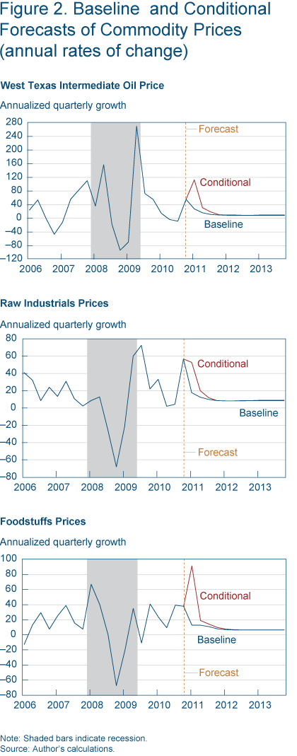
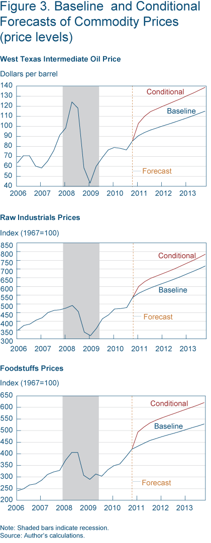
Although commodity prices were already on the rise in the fourth quarter of 2010, the baseline simulation indicates that the increase was expected to slow in the first quarter of 2011. For example, after averaging $85 per barrel in the fourth quarter, the price of WTI crude oil was expected to average $90 per barrel in the first quarter, according to the baseline simulation. The first-quarter average price came in $13 higher at $103 per barrel (roughly 15 percent). Interestingly, the BVAR model turned out to be an excellent predictor of the futures prices for WTI crude during this time. The two-month contract in mid-to-late December averaged roughly $90—nearly identical to the expectation generated by the BVAR baseline forecast.

Figure 2 compares the baseline (unconditioned) and alternative (conditional) forecasts of commodity prices, expressed in annual rates of change. Baseline first-quarter expectations undershot for all three commodity-price concepts in the model—quite drastically on all counts. Beyond the first quarter, the gaps between commodity-price growth rates in the conditional and baseline forecasts rapidly evaporate and return to trend growth paths. But figure 3, which plots the level of commodity prices instead of their rates of growth, makes it clear that there is no “correction” for the first-quarter shocks, meaning that commodity prices are permanently higher in the conditional forecast. A return to baseline commodity-price levels would require periods of falling commodity prices in the wake of the first-quarter shocks.

• 2a: West Texas Intermediate Oil Prices
• 2b: Raw Industrials Prices
• 2c: Foodstuffs Prices 

• 2a: West Texas Intermediate Oil Prices
• 2b: Raw Industrials Prices
• 2c: Foodstuffs Prices 

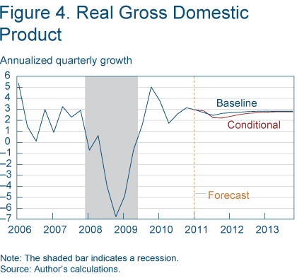
But what are the consequences of these price effects for real activity and inflation? Figures 4 and 5 indicate that all goes according to the principles: Beginning in the second quarter, real GDP growth falls and inflation rises, but by fairly modest amounts in both cases. Figure 4 shows that the maximum reduction in real GDP growth (annual rates) is just 0.4 percentage point, occurring in the fourth quarter of 2011; the gap between the two forecasts steadily closes thereafter. As for inflation, figure 5 shows that PCE inflation (annual rate) jumps 0.7 percentage point (from 1.5 percent to 2.2 percent) in the second quarter of 2011 and shows more persistence than real GDP, as it returns only gradually to the baseline forecast.

 

 

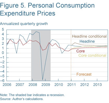
The sharp response of PCE inflation is due to the rapid pass-through of energy and food commodity prices into consumer energy and food prices. Most auspiciously, the price of gasoline to the consumer responds quickly to changes in crude oil prices. Indeed, core PCE inflation, or inflation excluding food and energy prices, rises a more muted 0.3 percentage point by the fourth quarter of 2011 (from 1.1 percent to 1.4 percent), reflecting the limitations confronted by firms in passing on higher commodity costs to consumers.

The Bottom Line

In summary, the analysis indicates that the shocks we experienced in the first quarter of 2011 have had measurable effects on both economic activity and consumer price inflation. However, as long as energy and other commodity prices do not continue to rise sharply, these effects are likely to be temporary and modest.