

- Share
Why Are Headline PCE and Median PCE Inflations So Far Apart?
Mean (or headline) PCE inflation has typically fallen below median PCE inflation, and since 2012 the difference has been large. To understand the reasons for this trend, we investigate which components of the headline measure are contributing to the difference. We find that energy components, which frequently undergo wide price swings, and electronics, which have been steadily decreasing in price for decades, explain most of the difference between the two inflation measures. We argue that the outsized impacts of such components on headline PCE inflation reinforce the need for policymakers to consider both headline and median PCE inflation measures.

The views authors express in Economic Commentary are theirs and not necessarily those of the Federal Reserve Bank of Cleveland or the Board of Governors of the Federal Reserve System. The series editor is Tasia Hane. This paper and its data are subject to revision; please visit clevelandfed.org for updates.
The Federal Reserve has a mandate from Congress to maintain price stability in the economy. To this end, the Federal Open Market Committee (FOMC) targets a 2 percent annual change in the personal consumption expenditure (PCE) price index. PCE inflation is calculated by tracking price changes in a basket of goods and services, the selection of which is designed to cover all possible expenditures consumers typically make. The central tendency of these price changes then represents the overall inflation in the economy.1
How best to measure this central tendency is debated among economists. The traditional method, known as headline PCE inflation, is simply to take a weighted average (mean) of all of the component price changes, with each item’s weight determined by its share of spending in the PCE basket. A less volatile alternative, core PCE inflation, is a weighted average of the nonfood and nonenergy components of the basket. And most recently, an even less volatile measure, median PCE inflation, has gained traction. It is calculated by taking the weighted median price change in the complete basket. Carroll and Verbrugge (2019) show that median PCE inflation does a better job of forecasting future inflation than either core PCE or headline PCE itself.2
Despite their shared intention of measuring the central tendency of the PCE basket, the median and headline PCE inflation figures have recently been quite far apart: According to the data available in late August, year-over-year median PCE inflation was at 2.5 percent while headline inflation was at a much lower 1.0 percent. Such a gap between the two measures is not uncommon: The high variability of headline compared to median PCE inflation can create considerable, sometimes persistent separation. Figure 1 shows that for the past eight years, headline PCE inflation has generally been much lower than median PCE inflation, leading to different signals about both the current level and the likely path of inflation. More importantly for policymakers, over that period the two measures have consistently provided different answers as to where inflation stands relative to the FOMC’s target rate: Headline PCE inflation has stubbornly remained below target, while median PCE inflation has been at or even well above the target.
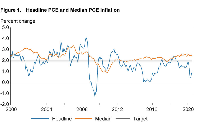
Source: Bureau of Economic Analysis, July 2020 PCE release.
A mean average that is well below the median indicates a negative skew in the distribution of component inflations: The components with price changes below the median tend to stray further from the median than those above.3 In this Commentary, we highlight several factors that account for a significant portion of the gap between the headline and median PCE inflation measures since 2012. Some of these components have had atypically low price growth during this period, and so we would expect them to correct over time and revert to their historical averages. Others have demonstrated long, consistent trends of negative price growth—referred to as secular patterns. These secular patterns have increased the skewness in the distribution of PCE prices such that the mean (headline PCE) tends to fall below the median (median PCE).
Why Median PCE Inflation Is a More Stable Measure Than Headline PCE Inflation
As mentioned, headline PCE inflation is constructed by taking a weighted average of the price changes for each component (good or service) in the PCE basket. The measure can be strongly affected by shocks in one component’s price, making it quite volatile. A component triggering a significant movement in the headline PCE will be driven either by its weight in the basket or by the magnitude of the price fluctuation associated with it. That is, a component with a disproportionate weight in the basket will count more in the calculation of mean average price growth, and a component with large year-to-year price fluctuations can have a significant effect on the mean average, even if it has a relatively low weight.
There are about 200 components in the PCE basket. If all components had equal weights, then each would count for 0.5 percent. But as the weight for each item is based upon its share of total household expenditures, items on which households spend the most get the most weight.
Table 1 reports the eight components with the greatest weights in the PCE basket. Notice that two components, owner-occupied stationary homes and tenant-occupied stationary homes, together comprise more than 15 percent of the total basket. This means that movements in housing inflation have roughly 30 times the effect that an average-sized component with the same price change has. However, sudden large movements in housing are rare: Since 2000, year-over-year housing inflation has been stable between 2 percent and 4 percent. Housing, then, does not explain the substantial swings in headline PCE inflation or the gap between headline and median PCE inflation; rather, housing should be thought of as a stabilizer for the headline measure. In fact, from 2013 to 2016, when headline PCE inflation dropped well below the 2 percent target rate, a small rise in housing inflation actually prevented it from dipping even further.
| Components | Share of total expenditures, percent |
|---|---|
| Owner-occupied stationary homes | 11.27 |
| Nonprofit hospitals’ services to households | 5.22 |
| Other purchased meals | 4.50 |
| Tenant-occupied stationary homes | 4.05 |
| Physician services | 3.98 |
| Prescription drugs | 3.08 |
| Final consumption expenditures of nonprofit institutions serving households | 3.07 |
| Gasoline and other motor fuel | 2.32 |
Source: Bureau of Economic Analysis. Last observation is from the July 2020 PCE release.
Contrast the behavior of housing with that of a small collection of components commonly lumped together in the energy category.4 One of those is gasoline and other motor fuel. At 2.3 percent of the PCE basket, it has a much smaller weight than housing but often has a vast effect on headline PCE inflation. It is able to exert such a large pressure because the price changes in gasoline are typically much greater in magnitude than the price changes in housing (see figure 2).
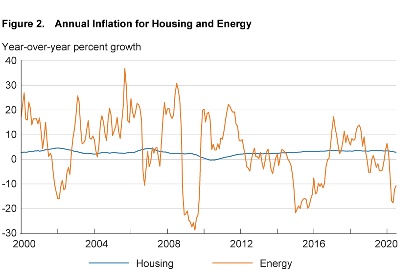
Source: Bureau of Economic Analysis, July 2020 PCE release.
The sensitivity of headline PCE inflation to outliers has motivated the exploration of other inflation measures that focus on the middle of the distribution of price changes across items, including the median PCE.5 Median PCE inflation, as the name indicates, uses a median average to measure inflation. This is accomplished by first sorting basket components according to their monthly price changes in increasing order, then calculating the cumulative weight of components in the newly ordered basket,6 and finally recording the price change of the component whose weight pushes the cumulative weight above 50 percent. By computing inflation in this way, median PCE inflation is not influenced by the magnitude of any price change that appears in one of the tails of the distribution. The fluctuations in median PCE, therefore, tend to be gradual and restrained compared to those in the headline measure, which is why it is not uncommon to observe temporary sizable discrepancies between headline and median PCE inflation.
What Is Behind the Persistent Gap between Median PCE and Headline PCE Inflation since 2012?
Figure 3 shows the difference in percentage points between median and headline PCE inflation since 1978. Throughout the period, headline PCE inflation tends to be lower than the median, and the magnitude of the difference between them undulates. Sometimes the period of separation can be lengthy, as it was during the extended spell of expansion in the 1990s. Sometimes the difference changes more sharply. For instance, the 2000s saw rapid swings in the difference between the inflation measures, likely in part catalyzed first by wars in the Middle East leading to shortages of crude oil and second the Great Recession from 2007 to 2009.
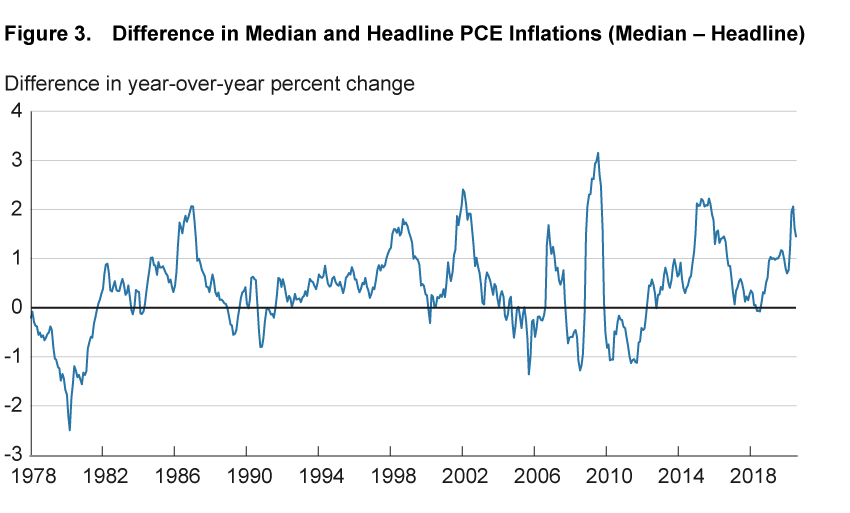
Source: Authors’ calculations based on data from the Bureau of Economic Analysis, July 2020 PCE release.
Of more immediate interest is the period since 2012, a prolonged episode during which headline PCE inflation has generally been much lower than median PCE inflation. As the discussion above indicates, this difference is likely due to items with relatively large weights that experienced extremely negative price changes. This motivates the following exercise: Identify the primary contributors to the gap by recalculating mean inflation using a restricted PCE basket in which one or more of the low-inflation components have been removed. As we remove components that are regularly negative-inflation outliers for 12-month stretches, the weighted mean inflation for this restricted basket, which we denote “restricted headline PCE” inflation, necessarily rises toward the median PCE measure, closing the gap. The removed components are then determined to be those responsible for the gap, and we examine them in more detail for clues about their individual patterns.
We begin by removing energy components, whose prices have been decreasing for a vast majority of the period since 2012. We know that energy can have a significant effect on headline PCE. For instance, in the years 2014 to 2016, when energy experienced a 20 percent year-over-year price drop, headline inflation dipped nearly to zero.7
Figure 4 shows headline PCE inflation with and without energy components in the basket. Once energy is removed, headline PCE inflation since 2012 becomes considerably more stable, and the gap between the two PCE inflation curves closes by an average of 0.19 percentage points. Nevertheless, the restricted basket’s inflation rate still mostly remains below the 2 percent target, and far below median PCE inflation, for nearly the entire period. Much of that has to do with items whose prices have shown steady downward trajectories. No category of components is more emblematic of this behavior than electronics.
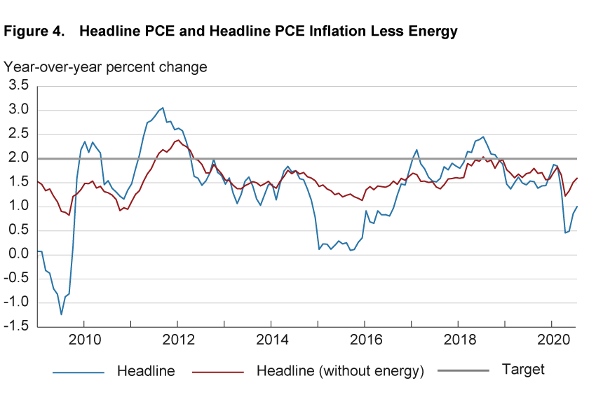
Source: Authors’ calculations based on data from the Bureau of Economic Analysis, July 2020 PCE release.
Electronics
Table 2 lists the 12 components of the PCE basket with an average yearly price decrease of at least 4 percent since 2012.8 Ten are in the electronics category.
| Component | Average inflation | Weight |
|---|---|---|
| Televisions | −16.3 | 0.25 |
| Telephone and related communication equipment | −15.2 | 0.22 |
| Calculators, typewriters, and other information processing equipment | −8.7 | 0.01 |
| Games, toys, and hobbies | −7.2 | 0.52 |
| Personal computers/tablets and peripheral equipment | −6.4 | 0.40 |
| Exchange-listed equities | −5.9 | 0.02 |
| Audio equipment | −5.8 | 0.16 |
| Clocks, lamps, lighting fixtures, and other household decorative items | −5.4 | 0.30 |
| Cellular telephone services | −5.4 | 0.96 |
| Computer software and accessories | −5.0 | 0.59 |
| Video discs, tapes, and permanent digital downloads | −4.5 | 0.10 |
| Other video equipment | −4.2 | 0.12 |
Source: Bureau of Economic Analysis. Last observation is from the July 2020 PCE release.
Examining the time series of each of these components’ inflations more closely, we find that most had consistent negative price growth over the entire period. In other words, their low averages are not attributable to irregular, extreme 12-month price drops, as seen in energy, but rather to a systematic downward trend. For example, figure 5 plots the year-over-year inflation rates for the first four components in table 2. Notice that over the period, the inflation rates are always negative, which means that their price levels are always dropping. The components in table 2 are generally those most heavily impacted by improvements in technology. On the supply side, cheaper production costs can lower prices, while on the demand side, newer models render the older ones less desirable, likewise lowering prices.
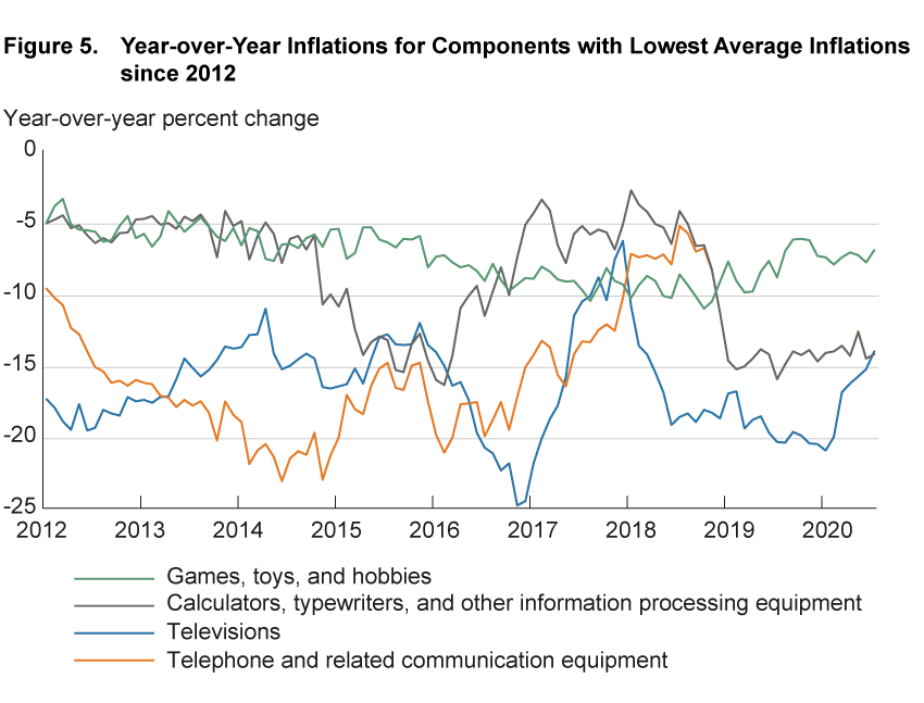
Note: From January 2019 on, the data for telephones and related communications equipment are very similar to those for calculators, typewriters, and other information processing equipment, so the plotted lines for these two series overlap on the chart.
Source: Bureau of Economic Analysis, July 2020 PCE release.
The deflationary nature of electronic items need not mean consumers are spending less on them. Electronics are always improving, and to make meaningful comparisons of price changes over time, those improvements in quality have to be figured into the calculations of the indexes. To calculate price indexes, the Bureau of Economic Analysis (BEA) controls for quality changes using composite methods (Moulton, 2001). When a full sample of prices is available across two periods, the BEA employs a matched-model method—that is, it calculates the price changes within product models to determine the overall component price change. Televisions, for instance, saw remarkable price decreases in the latter 2000s. High-definition TVs took over the market, which drastically lowered the value of standard-definition TVs. Eventually, most standard definition TV models became obsolete, leaving a void that biases inflation rates based on matched-model methods upward. To account for changes in the market, the BEA then employs hedonic methods to prescribe value to the quality improvements of newer models. It calculates price indexes by subtracting out the estimated value of the quality improvements.9 Because electronics are rapidly improving, after quality adjustment, their measured price changes from inflation are actually negative.
When we remove electronics, whose price declines have consistently pulled headline PCE inflation down over the last eight years, as well as energy, whose volatility tends to pull the mean away from the median, over half of the average gap between the headline and median PCE inflation curves since 2012 disappears. Figure 6 and table 3 demonstrate this effect.
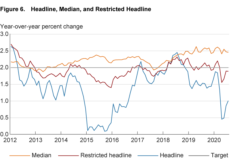
Source: Authors’ calculations based on data from the Bureau of Economic Analysis, July 2020 PCE release.
| Restrictions | Average gap (in percentage points) |
|---|---|
| Unrestricted | 0.83 |
| Energy removed | 0.64 |
| Energy and electronics removed | 0.35 |
Source: Authors’ calculations based on data from the Bureau of Economic Analysis. Last observation is from the July 2020 PCE release.
What Is Causing the Gap Today?
From March to July 2018, year-over-year headline PCE and median PCE inflation were nearly identical. This marked the end of a prolonged episode in which headline inflation had run far below the median measure. Since that time, a gap has reemerged, as the headline measure has fallen below the FOMC’s target and the median has risen to 2.5 percent year-over-year. Once again, policymakers are faced with conflicting signals.
As we did for the full period since 2012, we can again remove components to uncover which are most responsible for creating the separation after July 2018. Energy and secular components (again, predominantly electronics) continue to have a sizable combined effect, accounting for on average 0.47 percentage points of the gap.
That just a few components can have such an outsized effect on headline PCE inflation compared to median PCE inflation is not by itself a problem. In fact, the headline measure can offer critical insight that the median may not pick up, such as dramatic price drops in a few industries. However, this focus on the tails of the inflation distribution may paint an incomplete picture of the economy, which is why incorporating the median PCE measure into inflation analysis can be useful, bearing in mind that the presence of secular components will on average depress the mean more than the median.
A Note on the Effects of the COVID-19 Pandemic
COVID-19 and the social-distancing policies aimed at slowing the spread of the virus have exerted a deflationary force on weighted-average price indexes. In particular, components related to travel were subject to dramatic price drops, as businesses struggled to sell excess supply. Motor fuel prices, which had been rising slightly prior to the pandemic, started to decrease dramatically in February 2020, culminating in a 94 percent annualized price drop in April.10 Motor vehicle rentals, air transportation, and hotels also experienced major price depression. Furthermore, prices broadly decreased in a host of other categories including clothing, entertainment, and, as per usual, electronics. Annualized headline PCE inflation was −6.4 percent for the month of April, the lowest monthly inflation rate since the Great Recession.
Simply put, the headline PCE inflation figure for April tells of something drastic taking shape in the economy. The same cannot be said of the median PCE, whose annualized reading for April of 2.1 percent is hardly an outlier. Each measure offers its own insight: We notice that the center of the component inflation distribution remains stable while the vast movement occurs in the left tail. As we discussed, variation in the gap between headline and median PCE inflation is attributable to idiosyncratic components whose prices can fluctuate tremendously and visibly move the headline measure even if they have small weights. This effect has been particularly pronounced during the pandemic: Many of the components with the largest decreases in price also carried abnormally small weights due to decreased demand.11 Meanwhile, these components with extreme inflations impacted the median PCE reading only insofar as they moved from the positive side of the center of component inflations to the negative side. And due to a robust center of the distribution, where inflation rates remained quite steady—including in housing and food items—the overall decrease in median PCE inflation is marginal.
Footnotes
- Annual inflation can be reported as annualized monthly inflation or as year-over-year price changes. The latter is used throughout this Commentary. Return
- Other studies have made a similar point using the consumer price index. See Bryan and Pike (1991), Bryan and Cecchetti (1993), and Meyer, Venkatu, and Zaman (2013). Return
- If we remove the top and bottom 5 percent of the component inflation distribution each month and then recompute year-over-year mean inflation since 2012, the gap between median PCE inflation and headline inflation decreases on average by 0.22 percentage points. Return
- The energy category is composed of the components gasoline and other motor fuel, lubricants and fluids, fuel oil, electricity, and natural gas. Return
- The Dallas Fed trimmed-mean is another prominent alternative inflation measure. Return
- Components are sorted from lowest inflation on the left to highest inflation on the right. Their weights are ordered accordingly. The cumulative weight for a given component is the sum of its weight and the weights of all components to its left. Return
- Likewise, from May to July 2018, the only stretch since 2012 in which headline PCE inflation has exceeded median PCE inflation, year-over-year energy inflation was positive too at roughly 13 percent. Return
- For comparison, the component gas and motor fuel fell by an average of 2 percent over this period. Return
- See https://www.bls.gov/cpi/quality-adjustment/questions-and-answers.htm for a more detailed explanation of how the method works using an example with televisions. Return
- The annualized inflation rate is the one-month inflation rate converted to a 12-month rate. Return
- In a counterfactual scenario in which consumption weights in April 2020 are replaced with those in April 2019, headline PCE inflation becomes −9.0 percent, 2.6 percentage points lower than the actual measure. In the months prior to the pandemic, using the weights from the previous year yielded negligible differences. Meanwhile, median PCE inflation is practically unchanged using the counterfactual weights. Return
References
- Bryan, Michael F., and Stephen G. Cecchetti. 1993. “The Consumer Price Index as a Measure of Inflation.” Federal Reserve Bank of Cleveland, Economic Review, 29(4): 15–24. https://fraser.stlouisfed.org/title/1328/item/4593/toc/153504.
- Bryan, Michael F., and Christopher J. Pike. 1991. “Median Price Changes: An Alternative Approach to Measuring Current Monetary Inflation.” Federal Reserve Bank of Cleveland, Economic Commentary, December 1. https://doi.org/10.26509/frbc-ec-19911201.
- Carroll, Daniel R., and Randal Verbrugge. 2019. “Behavior of a New Median PCE Measure: A Tale of Tails.” Federal Reserve Bank of Cleveland, Economic Commentary, 2019-10. https://www.doi.org/10.26509/frbc-ec-201910. https://doi.org/10.26509/frbc-ec-201910.
- Meyer, Brent H., Guhan Venkatu, and Saeed Zaman. 2013. “Forecasting Inflation? Target the Middle.” Federal Reserve Bank of Cleveland, Economic Commentary, 2013-07. https://doi.org/10.26509/frbc-ec-201305.
- Moulton, Brent R. 2001. “The Expanding Role of Hedonic Methods in the Official Statistics of the United States.” Bureau of Economic Analysis. https://ideas.repec.org/p/bea/papers/0018.html.
Suggested Citation
Carroll, Daniel R., and Ross Cohen-Kristiansen. 2020. “Why Are Headline PCE and Median PCE Inflations So Far Apart?” Federal Reserve Bank of Cleveland, Economic Commentary 2020-24. https://doi.org/10.26509/frbc-ec-202024
This work by Federal Reserve Bank of Cleveland is licensed under Creative Commons Attribution-NonCommercial 4.0 International

