

Zero Growth and Long-Run Inequality
Using a basic model to study both wealth and income inequality and their relations to long-run economic growth may lead to questionable conclusions. We consider a more complex model that includes realistic variation in the levels of income and wealth across households in addition to a new ingredient, luck in each household's labor productivity. Using this model, we determine that existing estimates of the elasticity of substitution between capital and labor are generally far away from the region where inequality would explode if long-run growth were zero.
Inequality in wealth and income has become an issue of frequent debate, for not only policymakers but also the general public. Recently, the discussion has drifted toward a particular question motivated in part by the Great Recession and ensuing slow recovery: does income inequality and wealth inequality increase as the economy’s long-run rate of economic growth slows? In this context, “long-run economic growth” refers to the positive trend in real economic variables such as output, consumption, and investment that can be attributed in part to the advancement in technology and to population growth. Research by Thomas Piketty and co-authors has answered the question above in the affirmative; however, their work relies on strong assumptions about how the wealth distribution evolves and how the economy produces output.
In a recent Federal Reserve Bank of Cleveland working paper, we explore the same question using modern macroeconomic models of income and wealth inequality, and we find that inequality is only weakly related to long-run economic growth. What relationship is there tends to be negative rather than positive: income and wealth inequality tend to be lower when the long-run growth rate is zero (i.e., when output remains the same over time).
The direction of this relationship depends critically upon the degree to which capital and labor are interchangeable in production. When they are strong substitutes for each other, inequality can become very extreme, exactly as Piketty describes. On the other hand, when capital and labor are less interchangeable or when they work together, as the empirical literature strongly suggests, long-run inequality is lower under zero growth. As a result, while concerns about income and wealth inequality are understandable and warrant discussion, extreme inequality is not the likely outcome of low economic growth because capital and labor are not strong substitutes.
In our analysis, we draw on modern macroeconomic models of inequality that include a sophisticated treatment of the distribution of income and wealth. In particular, our models naturally give rise to distributions of income and wealth that respond to economic forces and do not require restrictive assumptions about a particular distribution. In a simplified version of the model, we find that a near-zero rate of long-run growth causes extreme income inequality only in calibrations of the model that are inconsistent with empirical evidence. When we extend the model to include a more sophisticated treatment of income and wealth distributions, such as those found in real-world contexts, we find that zero growth has little effect on income and wealth inequality. In fact, to the extent that different rates of trend growth are associated with changes in wealth inequality, lower growth tends to yield less inequality rather than more.
Modeling Concepts
It is helpful to introduce some fundamental concepts from the economic model. The elasticity of substitution in production governs the ways in which capital and labor can be combined to produce the same level of output. If the elasticity is very high, then capital and labor are strong substitutes, meaning that one can swap out one input for another relatively easily and achieve the same amount of production. When the elasticity is very low, capital and labor are strong complements, meaning that they work together in production.
As an example of high elasticity of substitution, consider a factory that puts labels on cans. To produce 10,000 labeled cans in an hour, a company could use one labelling machine or 20 human labelers. The machine (capital) and the labelers (labor) do not need each other to function, so 20 labelers could be replaced by one machine, and the resulting output would be the same. For an example of low elasticity, think of a shipping firm that uses trucks to move goods across the country. More trucks (capital) means that more goods can be moved, but only if there are also more truck drivers (labor) to operate them.
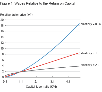
The elasticity of substitution governs the sensitivity of factor prices, that is, the wage and the rental rate (i.e., the return paid to a unit of capital) to imbalances in the ratio of capital to labor. The more that labor and capital are substitutes, the less factor prices adjust as one input to production becomes more abundant than another. However, if labor and capital are less substitutable, then the factor prices can be very responsive.
This idea is of particular importance when contemplating a world with extreme capital accumulation. In such an environment, capital would be very abundant relative to labor. Unless the two factors are very substitutable, the relative scarcity of labor would drive up wages relative to the rental rate. All else being equal, this relative rise in the wage would increase labor income relative to capital income and thus reduce income inequality. (See figure 1.)
We next turn to using these concepts in a relatively simple version of our model.
The Basic Model
Our models feature firms (businesses) and two types of households: laborers and capitalists. Firms produce output using labor and capital inputs. Output, measured by GDP, includes consumption and investment (the latter of which adds to the economy’s stock of capital). A laborer earns all income from working, while a capitalist can earn income both from working and from the returns on wealth.
To facilitate analysis, in the case of the basic model we make several simplifying assumptions. First, we fix the percentages of households that are laborers or capitalists. In particular, we make 20 percent of the households capitalists, roughly in line with the distribution of stock ownership in the United States. Second, we abstract from multiple children and inheritances: our model is one in which a parent has only one child and leaves a bequest to his or her heir upon death. Finally, we abstract from taxes on capital income and estates by setting them equal to zero. With this setup, the model makes it possible for capitalist households to build up large wealth positions, and thus, at least conceptually, there is potential for extreme levels of income inequality as capitalist households’ wealth increases and laborer households’ income fails to keep pace.
The key insight from this basic model is that in order for income inequality to become very large as the economy’s growth rate falls to zero, the elasticity of substitution between labor and capital must be well above 1, meaning that a percentage decrease in one of the inputs could be offset by the same percentage increase in the other input and total output would be the same. If this elasticity is not sufficiently above 1, income inequality cannot become extreme. For example, if capital’s share of production is 36 percent (a widely used estimate in the research literature), the elasticity of substitution must be over 1.38 for income inequality to explode.
Existing estimates of the elasticity of substitution between capital and labor are generally far away from the region where inequality would explode if long-run growth were zero given any empirically reasonable value for capital’s share. In a summary of the literature, Chirinko (2008) writes that “the weight of evidence suggests that [the elasticity of substitution] lies in the range between 0.40 and 0.60,” suggesting that the return to labor relative to capital would increase fast enough as growth slowed to zero to offset the wealth accumulation of capitalist households. Table 1, taken from Rognlie (2014), summarizes the results from the 31 studies examined in Chirinko (2008).
| Elasticity | Number of studies |
|---|---|
| 0–0.49 | 14 |
| 0.50–0.99 | 12 |
| 1.00–1.49 | 3 |
| 1.50–1.99 | 1 |
| 2.0–4.00 | 1 |
What is the intuition for these findings? At zero long-run growth, capitalists save a lot of wealth; however, under most parameterizations of the model, this behavior does not produce a big rise in income inequality because the wage and the return to capital adjust to supply and demand. As capitalists save more and more, capital becomes very abundant relative to labor, causing the return on capital to plummet relative to the wage. As a result, capital income, which is the product of wealth and the return to capital, does not increase. In some cases, it may even fall. It is only when we specify the model so that capital and labor are strong substitutes in production, and hence the ratio of wages to capital returns is not very responsive to the great relative abundance of capital, that we can get explosive income inequality.
A More Sophisticated Model
While the basic model captures the fundamental concepts, it is too simple to address questions involving wealth inequality since, by construction, 20 percent of the population—the fixed share of capitalists among households—always owns 100 percent of the wealth in the economy. Moreover, there is no scope for wealth heterogeneity among capitalists. In order to study both wealth and income inequality, we consider a richer, more complicated version of the model, one that allows meaningful distributions of both income and wealth.
To get more realistic variation in the levels of income and wealth across households, the extended model adds a new ingredient: luck in each household’s labor productivity. Using this model, changes in productivity translate one-for-one into changes in wages. In every model period, each household draws a “shock” to its productivity (wage) from a random process. Some households will receive good surprises, others bad ones. Households respond by saving for a rainy day: in periods of high wages they build up precautionary savings, to be ready for future periods in which their wages may be low, to avoid large cuts in their consumption. In order to maintain our capitalist/laborer dichotomy, and to allow for the possibility of extreme inequality, we assume the return on savings by laborers is lower than the return on capital. Because the return on savings is relatively low for laborers, they will not amass any more wealth than is necessary for their precautionary saving.
This model delivers distributions with a wide range of income and wealth, like those in the real world. This permits us to describe and quantify inequality with standard tools such as the Lorenz curve and the Gini coefficient. (See box.)
It turns out that wage risk has little effect on the evolution of long-run income and wealth inequality as growth falls to zero in the model. Even though the amount of capital in the economy increases, the return on that capital declines, preventing a large run-up in income inequality. In fact, wealth inequality in the model as measured by the Gini coefficient actually falls slightly, from roughly 0.85 to 0.84. The reason for this is that many capitalists save enough wealth that they no longer work. Once they stop working, fluctuations in their (potential) wage have very little effect on their behavior. By amassing a large buffer of savings, they insulate themselves from risk. In this richer model, what would it take to have extreme inequality? This model as described above cannot produce extreme inequality.
To see if we can get higher model-based inequality than described above, we modify the model to include two more ingredients. First, we add some risk into each capitalist’s return. As with the wage shocks, within each period some capitalists do better than average in the market, while others do worse (some start Google, others start 1990’s startup Pets.com). Because the return to capital is now risky, capitalists will limit their savings, so they will not get as wealthy as they would with no return risk. Second, we change the economy’s production function to include technology change that is biased toward capital, meaning that over time capital becomes more important than labor in production; this force drives up the return on capital relative to labor.
Together, reducing return risk and increasing capital’s return relative to labor offers the strongest opportunity for zero growth to generate large increases in income and wealth inequality. Reducing return risk induces capitalists to save more, while technical change that is biased toward capital acts to prevent declines in returns—the net result is that both components of capital income can rise. However, even with the two factors biasing our results toward high inequality, the model does not predict exploding inequality. The Gini coefficient on wealth declines, this time from 0.97 to 0.89 so that once again zero growth implies lower inequality rather than greater inequality.
Conclusions
Despite concerns that declining growth rates will lead to ever-increasing wealth and income inequality, modern macroeconomic models do not predict that this explosion will occur unless capital and labor are far more substitutable in production than data suggest. Research that has relied on models designed for studying only the behavior of macroeconomic aggregates and that do not contain endogenous income and wealth distributions can be misleading, as these models tend to “bake in” the results from the start instead of permitting them to emerge naturally. Household income and wealth heterogeneity remains a very active area of research in economics. A fuller understanding of all forces shaping inequality will offer insight into a wide range of economic issues and lead to better policy in the future.
Computing the GINI Coefficient
Box 1. Computing the Lorenz Curve and Gini Coefficient
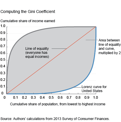
To construct a Lorenz curve, we rank households according to their wealth; the Lorenz curve plots the fraction of total wealth that is held by households who are poorer than a given fraction of the population. If the curve lies on the 45-degree line, then wealth is equally distributed. The farther the Lorenz curve drops below the 45-degree line, the more unequally wealth is distributed. In the extreme, where a single household owns everything, the Lorenz curve forms a right angle.
The Gini coefficient is an easy way to summarize a Lorenz curve. It is twice the area between the 45-degree line and the Lorenz curve. Under perfect equality, the Gini coefficient is zero. When a single household owns everything, the Gini coefficient is one. In the figure below, we plot the 2013 wealth Lorenz curve for the US.
References
- Carroll, Daniel, and Eric Young, 2014. “The Piketty Transition,” 2014. Federal Reserve Bank of Cleveland, working paper, no. 14-32.
- Chirinko, Robert S., 2008. “[Sigma]: The Long and Short of It.” Journal of Macroeconomics, vol. 30, issue 2.
- Piketty, Thomas, and Emmanuel Saez, 2014. “Inequality in the Long Run,” Science.
- Piketty, Thomas, and Gabriel Zucman, 2014. “Wealth and Inheritance in the Long Run.” Manuscript.
- Rognlie, Matthew, 2014. “A Note on Piketty and Diminishing Returns to Capital.” Manuscript.
The views authors express in Economic Commentary are theirs and not necessarily those of the Federal Reserve Bank of Cleveland or the Board of Governors of the Federal Reserve System. The series editor is Tasia Hane. This work is licensed under a Creative Commons Attribution-NonCommercial 4.0 International License. This paper and its data are subject to revision; please visit clevelandfed.org for updates.
Suggested Citation
Carroll, Daniel R., and Eric R. Young. 2015. “Zero Growth and Long-Run Inequality.” Federal Reserve Bank of Cleveland, Economic Commentary 2015-11. https://doi.org/10.26509/frbc-ec-201511
This work by Federal Reserve Bank of Cleveland is licensed under Creative Commons Attribution-NonCommercial 4.0 International


- Share