Labor Market Tightness across the United States since the Great Recession

Even though the Great Recession might feel like a distant memory, the episode’s effects on the labor market were so severe that they will be studied for some time to come. The unemployment rate, which hovered around 4.5 percent right before the start of the recession, jumped to 10 percent by its end and then stayed above 7 percent for the next four years. Focusing on the national figure, however, disguises the variation in rates that occurred at the state level. For example, when aggregate unemployment hit 10 percent in October 2009, Michigan’s unemployment rate was 14.2 percent, whereas North Dakota’s was only 4 percent.

In this Commentary, we explore this heterogeneity across states during and after the recession. To gauge the state of the labor market, we focus on labor market tightness. To measure tightness, we use the ratio of two common measures, the number of unemployed workers and vacancies. We demonstrate that the ratio is correlated with the business cycle and is thus a good measure of the state of the labor market. We map the evolution of the ratio over time in each state to show geographical variation in the intensity of the recession’s effects and the strength of the recovery.

Measuring Labor Market Tightness

The unemployment rate is arguably the most important summary statistic for the labor market. The numerator--the number of unemployed workers--measures the stock of available workers who are willing to work (and searching for employment), and as such, it indicates the level of unused human resources in the economy. The measure is calculated from data gathered by the Bureau of Labor Statistics (BLS) in its monthly household survey. Vacancies, on the other hand, are a measure of the other side of the market and give the number of unfilled job openings for which firms are willing to recruit. The vacancy measure we use comes from the Conference Board, which tracks help-wanted ads that are posted online. One appealing feature of these data is that they allow us to measure vacancies at the individual state level.

Combining these two indicators into one metric, the number of unemployed workers per vacancy (U/V), provides an intuitive way of summarizing the state of the labor market and is also a good cyclical indicator. Intuitively, when the U/V ratio is high, many workers are competing for a few job opportunities, a situation which occurs during recessionary episodes in the labor market. In contrast, when the ratio is low, firms are competing for fewer unemployed workers, raising the odds of workers finding jobs but making it harder to fill each vacancy on average. This is usually the case during an expansion. Theoretical models of labor markets that aim to understand fluctuations over the business cycle refer to V/U (the inverse of the U/V ratio) as “labor market tightness” and show that the variable is able to summarize the state of the labor market.¹ More recently, empirical work has shown that this tightness indicator underlies much of the volatility in the labor market in the aggregate data and is potentially driven by a single underlying factor (Hall and Schulhofer-Wohl, 2017).

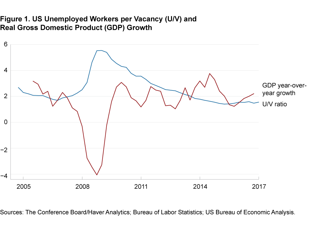
When we plot the U/V ratio, we can see that it seems to be countercyclical, rising during the recent recession and coming down during the recovery (figure 1). In addition, in other calculations, we find that negative rates of output growth are associated with a rising U/V ratio from 2005 to the present (the period for which we have data). As the economy recovers from the downturn, with higher demand for new workers, vacancies rise. Simultaneously, there are fewer separations among employed workers; hence, unemployment declines. As a result, the U/V ratio declines toward its normal level, that is, a level that is consistent with the average amount of turnover that occurs even in a healthy economy.

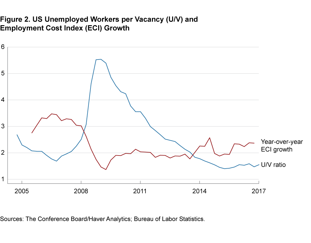
Plotting the U/V ratio against wage growth as measured by the employment cost index (ECI) provides insight into the relationship between labor market tightness and wages. Annual wage growth as reflected in the ECI starts declining as the number of unemployed workers per vacancy rises at the onset of a recession (figure 2). However, the reverse process is not symmetrical: As the labor market recovers and the U/V ratio declines, initially there is not much movement in the ECI until the U/V ratio converges to its prerecession level. This pattern suggests that it is plausible that firms do not need to bid up wages until they have strong competition for workers, that is, until the level of the U/V ratio is relatively low.

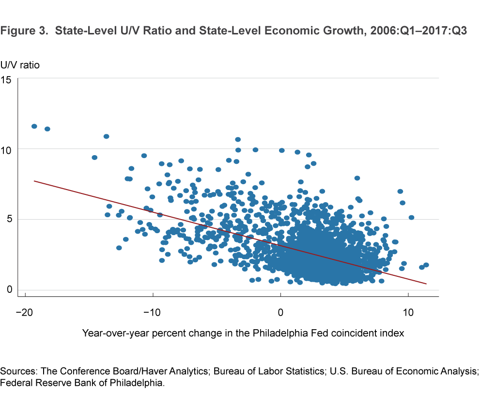
We argue that the countercyclical nature of the U/V ratio carries over to the state level. To show this, consider the correlation between state-level U/V ratios and a quarterly measure of economic activity at the state level, namely the coincident activity index produced by the Federal Reserve Bank of Philadelphia. This index measures the level of economic activity at the state level, much like the aggregate GDP does for the United States. As with the national U/V ratio and aggregate GDP, there is a robust negative correlation between the states’ U/V ratios and growth in economic activity at the state level (figure 3). The correlation coefficient between these two variables is between −0.5 and −0.81 for all but four states during the 2006:Q1–2017:Q3 period, pointing to strong countercyclical behavior. We estimate that 5 percent growth in economic activity during a year reduces the number of unemployed workers per vacancy by 0.55.²

Figures 1, 2, and 3, taken together, point to a highly cyclical U/V ratio. Along with the theoretical appeal, the empirical results lead us to believe that we can use the behavior of the U/V ratio at the state level to understand the evolution of the labor market throughout the business cycle.

Mapping the Recession and the Recovery

To understand the spatial distribution of the effects of the recession on the labor market, we show the intensity of market tightness over time in each state by plotting the U/V ratio on a map of the continental United States (figure 4). We want to summarize the state of the labor market in each state with just one number, so we show the U/V ratios in the month of June over two-year episodes starting in 2007. As we have explained above, the U/V ratio (unemployed workers per vacancy) shows how “good” the labor market is from the perspective of an unemployed worker. If the ratio is high, it indicates an abundance of unemployed workers competing for available jobs. As such, high ratios indicate lower odds of finding a job for the average unemployed worker. In rare cases, there could be more vacancies than unemployed workers (a ratio less than 1), indicating that firms are competing for unemployed workers.³

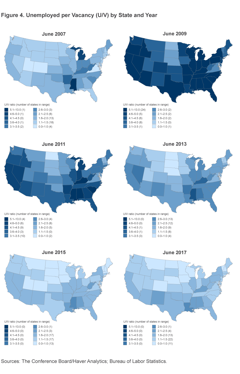
In June 2007, six months before the start of the recession, about 70 percent of the states had at most 2 unemployed workers per vacancy, with three states (Utah, Colorado, and Virginia) and Washington DC having at most 1 unemployed worker per vacancy. Parts of the Midwest (Michigan, Ohio, Indiana, West Virginia, Kentucky, and Missouri) and some southern states (Mississippi, Alabama, Arkansas, and South Carolina) stood out with more than 2.5 unemployed workers per vacancy. Hence, even before the recession, unemployed workers in some states were facing relatively unfavorable conditions. In the final month of the recession, June 2009, U/V ratios were high in almost every state, reflecting the severe effects of the recession. Half of the states had at least 5 unemployed workers for every vacant job opening in the state, and in one state, it was as high as 12 unemployed workers per opening (Michigan). Only states rich in natural resources (South Dakota, North Dakota, Alaska, and Nebraska) and states with relatively heavy federal government employment (Maryland, Virginia, and Washington DC) were spared the brunt of the recession to some extent and kept this ratio below 3.

By June 2011, two years after the end of the recession, areas in the Midwest and the sunshine states that had experienced significant problems in the housing sector still had more than 4 unemployed workers per vacancy. The rate for the median state was at 3.4, double the level in 2007. As the expansion of the US economy continued gradually, geographical imbalances dissipated somewhat, as can be seen in the snapshots for 2013, 2015, and 2017. Eventually, by 2017, only seven states had unemployment per vacancy levels higher than 2, a remarkable improvement relative to 2009. None of these states are in the North. The median rate came down at this point to 1.4 (Michigan), still lower than the 2007 level.

In some cases, more idiosyncratic reasons drive the labor market adjustment at the state level. North Dakota, for instance, had a very low U/V ratio over the entire period, seeming to be almost disconnected from the national business cycle in this sense. The state had a boom in the production of shale oil around this time, creating significant opportunities for employment in that sector and supporting service jobs. According to the Bureau of Economic Analysis, North Dakota ranked thirty-first among US states in its per capita gross domestic output in 2007 (at $44,585 in 2009 dollars). It experienced a meteoric rise to sixth place by 2016 because of the shale boom, with per capita GDP standing at $62,837 (in 2009 dollars). This natural-resource-driven growth more than offset the effects of the recession on the state economy, thereby keeping a relatively high demand for labor throughout the decade starting in 2007. A clear manifestation of this appears in North Dakota’s U/V ratio during our sample period. The unemployment rate fluctuated only between 2.5 percent and 4.3 percent (relatively low levels by any metric) during the past decade.

Conclusion

The Great Recession severely affected the aggregate US labor market, but experiences at the state level were not uniform. In order to gauge the dynamics of the labor market at the state level over time, we use the U/V ratio, which we argue is a good measure of the state of the labor market, presenting a robust correlation with the business cycle. Our analysis of the evolution of the U/V ratio over time within states shows that they charted different paths. Our maps show that the intensity of the adverse effects from the recession and the strength of the recovery varied geographically at all points in this process. Midwestern states, for instance, started with much more labor market “slack” than the average US state prior to the recession, but the states improved significantly during the decade.

References

- Pissarides, Christopher A., Equilibrium Unemployment Theory. MIT Press, Cambridge, 2000.
- Hall, Robert E., and Sam Schulhofer-Wohl. “The Pervasive Importance of Tightness in Labor-Market Volatility.” Unpublished manuscript, April 2017.
Suggested Citation
Tasci, Murat, and Caitlin Treanor. 2018. “Labor Market Tightness across the United States since the Great Recession.” Federal Reserve Bank of Cleveland, Economic Commentary 2018-01. https://doi.org/10.26509/frbc-ec-201801
This work by Federal Reserve Bank of Cleveland is licensed under Creative Commons Attribution-NonCommercial 4.0 International