Policy Rules in Macroeconomic Forecasting Models

In public discourse on the future course of the federal funds rate, the Taylor rule serves as a very common benchmark. According to the conventional Taylor rule, the target federal funds rate should increase as inflation rises above target or GDP rises above the economy’s potential level of GDP. The Taylor rule is popular for its simplicity—it includes only two variables—and for effectively capturing the history of monetary policy since the late 1980s.

Motivated by the prevalence of the Taylor rule as a benchmark and the potential for the rule to enhance our assessments of appropriate policy, this Commentary describes how some of the Cleveland Fed’s macroeconomic forecasting models (see Beauchemin 2011 for a description of one of them) have been modified to use a Taylor rule for monetary policy. These modifications require using sophisticated estimation techniques to simplify the federal funds rate equation of the model. After briefly describing the Taylor rule implementation, the article shows that the Taylor rule included in one of our models successfully captures the course of monetary policy in the most recent episode of policy tightening.

Taylor Rule Implementation

While many different versions of the Taylor rule have been proposed, the version originally proposed by John Taylor in 1993 is probably the best known:

Equation 1

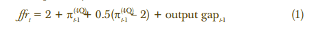
For the purposes of this analysis, ffr_t denotes the federal funds rate in the current quarter; the intercept of 2 captures the normal level of the real interest rate; inflation () is measured on a four-quarter basis with the core PCE price index; the inflation target is assumed to be 2 percent; and the output gap is the percent difference between actual GDP and potential GDP.¹ While the form of the rule in equation (1) is very common, there are other versions that are regularly used in research and policy analysis. To make the Taylor rule work effectively in our own forecasting analysis, we adopted some of the modifications that other researchers and analysts have proposed. In particular, we use the following form of a Taylor rule:

Equation 2

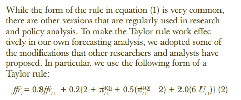
In this version, for both operational and conceptual reasons, we replace the output gap of equation (1) with an unemployment gap. This gap is defined as the long-run normal level of unemployment, currently estimated by Tasci and Zaman (2010) to be about 6 percent, less the actual unemployment rate last quarter (U_t-1).² In many economic models, the unemployment gap is closely related to the output gap: output above potential is associated with unemployment below its long-run or potential level. Operationally, our forecasting models don’t naturally yield an output gap, because they do not include the potential level of GDP. However, the models do include the unemployment rate. It is easier to combine the unemployment rate with an estimate of its long-run normal level to obtain an unemployment gap for the policy rule than to obtain an output gap.

Using unemployment also has some conceptual appeal. Although both unemployment and the output gap are very useful economic indicators, unemployment is more directly linked to the maximum employment component of the Federal Open Market Committee’s (FOMC) dual mandate (price stability is the other component).

To ensure our forecasting models provide an effective fit of historical data on the federal funds rate and other model variables, we modify the Taylor rule to include last quarter’s level of the federal funds rate on the right-hand side of equation (2).³ In models such as ours, which are vector autoregressive and estimated with Bayesian methods, the past level of the federal funds rate has considerable explanatory power for the current level. While this aspect of federal funds rate behavior may reflect several different forces (see, for example, Rudebusch 2006), one common view is that the FOMC has deliberately chosen to adjust the federal funds rate gradually. A commonly cited reason is that uncertainty about the effects of policy on the economy and uncertainty about the state of the economy warrant the gradual adjustment of policy (see, for example, Bernanke 2004).

The rule of equation (2) takes a form consistent with gradual adjustment. The rule sets the federal funds rate at a weighted average of last quarter’s federal funds rate (with a coefficient of 0.8) and a medium-term target (with a coefficient of 0.2). The medium-term target (the term in brackets on the right-hand side) corresponds to the prescription of the simple Taylor rule without gradual adjustment.

Finally, our Taylor rule of equation (2) reflects particular choices for the key coefficients of the rule—the coefficients on the past quarter’s federal funds rate, the deviation of inflation from trend, and the unemployment gap. To make the behavior of policy consistent across our models, we have opted to fix the coefficients at the values shown above instead of estimating them. We chose these values to be consistent with coefficients commonly used in other studies, often on the basis of Taylor rule estimates. In particular, we set the coefficient on last quarter’s federal funds rate at 0.8, consistent with estimates in such studies as Rudebusch (2006). The coefficient on the deviation of inflation relative to the target is set to 0.5, the value originally proposed in Taylor (1993), which remains a standard in other work with Taylor rules. We set the coefficient on the unemployment gap at 2.0, on the basis of recent estimates of unemployment-based Taylor rules (see Rudebush (2009) and Carlstrom and Lindner (2012)).⁴

The Rule’s Fit in a Historical Episode

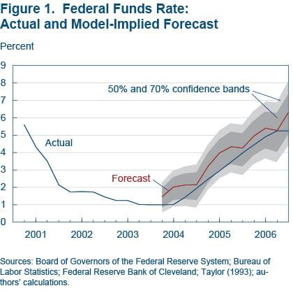
As a check on the consistency of the rule with historical policy (and an illustration of the type of guidance the rule may provide over the next few years), consider the rule’s prescriptions during the most recent episode of policy tightening. The episode is 2004:Q1 through 2006:Q4, when the FOMC raised the target federal funds rate from 1.0 percent to 5.25 percent.

To obtain these prescriptions, we use the model to generate a forecast of the federal funds rate over the period. The forecast is conditioned on the actual values of all of the other variables in the model, including inflation and the unemployment rate. The model, as mentioned above, is a vector autoregressive model, and the variables include GDP growth, the unemployment rate, core PCE inflation, headline PCE inflation, the spread between the BAA corporate bond yield and the 10-year Treasury yield, and the federal funds rate.⁵

The forecast corresponds to the path the federal funds rate would have most likely followed (according to the model), given the evolution of inflation, unemployment, and other model variables from 2004 through 2006.⁶ The estimated path takes into account the historical interaction among the federal funds rate and all the other variables of the model.⁷ If the rule were to perfectly describe the FOMC’s policy decisions during the period, the forecasted federal funds rate would coincide exactly with the actual federal funds rate. Of course, we don’t expect the rule to perfectly capture policy. Rather, we want to be sure the rule yields a funds rate forecast that is reasonably close to the actual path of the federal funds rate.

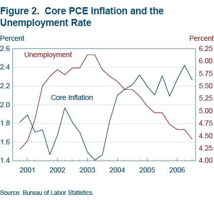
The results of the experiment confirm that the version of the Taylor rule incorporated in the forecasting model does a reasonably good job of capturing policy during the 2004–2006 episode (figure 1).⁸ The policy rule in the model yields a path similar to actual policy—broadly, a steady, substantial tightening of policy in response to increases in inflation and reductions in unemployment. In late 2003, with core inflation well below 2 percent and the unemployment rate down only slightly from its post-recession peak (and the economy still in a jobless recovery), policy was highly accommodative, with a federal funds rate target of 1 percent. As inflation picked up and unemployment declined in 2004 (figure 2), the FOMC began to gradually raise the federal funds rate. The Committee continued to steadily increase the federal funds rate in 2005 and 2006, as core inflation continued to drift up and unemployment trended down.

While the forecasted federal funds rate is above the actual funds rate for much of the period, the gap is small. In particular, it is well within the 50 percent confidence bands that reflect the historical uncertainty surrounding the predictions of the federal funds rate.⁹

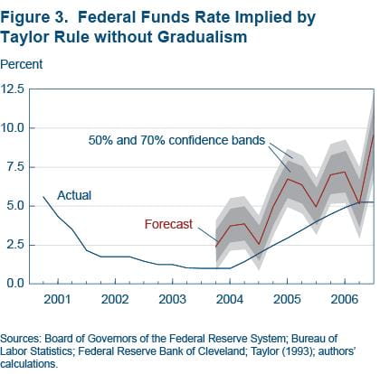
In light of the prominence of a simple Taylor rule without gradualism as a benchmark for appropriate policy, it makes sense to check how using a rule without gradualism in our forecasting model would fare in capturing policy during this episode. For this purpose, we modify the Taylor rule of equation (2) to make the coefficient on the lagged federal funds rate zero (instead of 0.8) and the coefficient on the term in brackets 1.0 (instead of 0.2). We then re-estimate the model with this rule and generate a new forecast of the federal funds rate, conditioned on the course of inflation and unemployment (and other model variables) from 2004 through 2006.

As figure 3 shows, this rule without gradualism yields a poor fit of the historical path of monetary policy.¹⁰ The forecasted path of policy is much higher than the actual path, with the actual path of the rate actually falling below even a 70 percent confidence interval around the model-implied path.¹¹ This finding confirms the need for including past federal funds rates in a Taylor rule (as we do in equation (2)) in models like ours.

That said, a simple Taylor rule in the form of equation (1) could be more effective as a guidepost when forecasts of future inflation and unemployment are plugged into the rule, in lieu of inflation and unemployment rates from the most recent quarter. The reason is that forecasts are inherently less variable than actual inflation and unemployment. But such a forecast-based version of the rule is difficult to use in vector autoregressive forecasting models like ours.

Conclusion

Drawing on other research that has found that past monetary policy can be accurately captured with a Taylor rule, this Commentary describes how we have modified some of our forecasting models to implement a Taylor rule. As one example, the rule does an effective job of capturing the tightening of policy during the 2004–2006 period. Looking ahead, we expect the rule to be a useful guidepost in our forecasting and policy analysis.

References

- “Shocks and the Economic Outlook,” by Kenneth R. Beauchemin, 2011. Federal Reserve Bank of Cleveland, Economic Commentary.
- “Gaps versus Growth Rates in the Taylor Rule,” by Charles T. Carlstrom and Timothy S. Fuerst, 2012. Federal Reserve Bank of Cleveland, Economic Commentary.
- “Monetary Policy and the FOMC’s Economic Projections,” by Charles T. Carlstrom and John Lindner, 2012. Federal Reserve Bank of Cleveland, Economic Trends, May 17.
- “Real-Time Density Forecasts from BVARs with Stochastic Volatility, by Todd E. Clark, 2011. Journal of Business and Economic Statistics, vol. 29, pp. 327-341.
- “The Fed’s Monetary Policy Response to the Current Crisis,” by Glenn D. Rudebusch, 2009. Federal Reserve Bank of San Francisco, Economic Letter, no. 2009-17.
- “Monetary Policy Inertia: Fact or Fiction?” by Glenn D. Rudebusch, 2006. International Journal of Central Banking, vol. 2, no. 4, pp. 85-135.
- “Discretion versus Policy Rules in Practice,” by John B. Taylor, 1993. Carnegie-Rochester Conference Series on Public Policy, December 1993, pp. 195-214.
- “The Ins and Outs of Unemployment in the Long Run: A New Estimate for the Natural Rate?” by Murat Tasci, 2010. Federal Reserve Bank of Cleveland, working paper no. 1017-R.
- “Unemployment after the Recession: A New Natural Rate?” by Murat Tasci and Saeed Zaman, 2010. Federal Reserve Bank of Cleveland, Economic Commentary.
Suggested Citation
Clark, Todd E. 2012. “Policy Rules in Macroeconomic Forecasting Models.” Federal Reserve Bank of Cleveland, Economic Commentary 2012-16. https://doi.org/10.26509/frbc-ec-201216
This work by Federal Reserve Bank of Cleveland is licensed under Creative Commons Attribution-NonCommercial 4.0 International