Explaining Apparent Changes in the Phillips Curve: The Great Moderation and Monetary Policy

Observations that the Phillips curve may be deviating from historical norms are important to policymakers because deviations would imply that more or less output has to be sacrificed to achieve a permanent reduction in long-term inflation. But we argue that recent economic shocks and a shift in the Fed’s response to inflation may be leading economists to misestimate the curve.

Ever since it was introduced five decades ago, many monetary policymakers have turned to the Phillips curve for the information and predictions it provides about the behavior of inflation. The curve, a standard part of many macroeconomic models, attempts to capture the relationship between current inflation and past inflation, expected inflation, and the output gap (the difference between the economy’s actual and potential output). Some assumptions are usually made when estimating the curve, one being that current inflation is a function of past inflation (because it is a good proxy for inflation expectations) and the current level of the output gap.

Recent calculations of the curve indicate that two aspects of it appear to be deviating from historical norms. The degree to which current inflation depends on past inflation, referred to as inflation persistence, has declined, as has the slope of the curve, which expresses the degree to which current inflation depends on the output gap.

Both changes could have important policymaking implications because such changes imply that more output has to be sacrificed in order to achieve permanent reduction in inflation. Each of the declines increases what is known as the curve’s implied sacrifice ratio, which is defined as the cumulative change in the output gap associated with a permanent change in long-term inflation.

But estimating the Phillips curve is tricky. Besides having to proxy for factors that aren’t observable, like expected inflation, economists must deal with the fact that the curve can be hit by “markup shocks,” which complicate the curve’s estimation because they cause inflation and the output gap to move in ways that are opposite what the curve would ordinarily predict. To further complicate the curve’s interpretation, other recent economic developments are probably accentuating the effects of these shocks. These developments include the declining volatility of potential output and a shift in the central bank’s operating procedure, which has made it more of an inflation-targeter. We argue that is quite probable that economists have been misestimating the Phillips curve recently and that the underlying Phillips curve, and thus the sacrifice ratio, have not really changed significantly.

Changes in the Inflation Process

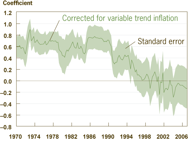
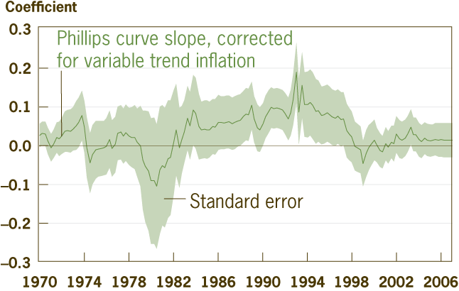
Figures 1 and 2 show why many think that the inflation process represented by the Phillips curve has fundamentally changed. These figures show estimates of inflation persistence and the slope of the Phillips curve since 1970 in rolling ten-year windows. We have corrected the estimates for changes in long-term inflation that may have occurred during this time period (For more detail see the Recommended Reading).

Notes: Inflation is based on unfiltered core PCE data. Coefficients are calculated using 10-year rolling regressions of inflation on the output gap and four-quarter lags of inflation. Inflation persistence is defined as the sum of the four-quarter-lag coefficients.
Sources: BEA; the Congressional Budget Office; authors’ calculations.

Notes: The output gap is defined as the natural log of real gross domestic product less the natural log of potential gross domestic product, taken from the Congressional Budget Office. Output gap coefficients are calculated using 10-year rolling regressions of unfiltered inflation data on the output gap and four-quarter lags of inflation.
Sources: Bureau of Economic Analysis; the Congressional Budget Office; authors’ calculations.

Around 1990 there was a rather dramatic decline in inflation persistence, from a value of roughly 0.7 to a value of zero (or even negative!) within the matter of a few years. A few years later, the slope of the Phillips curve flattened. Our corrected estimation of the curve suggests that the underlying relationships haven’t changed as much as people fear: the decline in the slope of the curve is not historically unusual. However, the magnitude of the decline in inflation persistence is.

Still, it is not clear that estimations of the Phillips curve tell us unequivocally that either inflation persistence or the relationship between inflation and the output gap has declined. Estimations of the Phillips curve, however, can be distorted by shocks to the curve itself.

Phillips Curve Basics

The kind of shock that complicates the estimation of the Phillips curve is a mark-up shock. These shocks are problematic because they manifest themselves as an increase in inflation and a decrease in the output gap (percent deviation of output from potential). To appreciate how such shocks have and continue to complicate the curve’s estimation, one needs to understand two assumptions that underlie the curve: imperfect competition and sticky prices. These assumptions provide the link between inflation and the output gap that is implied by the Phillips curve.

When markets are perfectly competitive and prices are flexible, prices are always equal to the marginal cost of production. The reason for this is clear when one considers what would happen if prices were higher than the marginal cost in such an environment. Each firm would have an incentive to expand its production by one unit, since the increased revenue from selling the product would be greater than the marginal cost of producing that unit. Each firm would find it in its best interest to increase production. The collective increase in production would push prices down (and/or the marginal cost up) until prices equaled marginal cost. Since the price of a product also measures the value consumers place on one more unit of the good, the fact that prices equal marginal cost means that output is at its socially efficient level.

But of course markets are not perfectly competitive. Instead, firms usually have some monopoly power and restrict production in order to charge a higher price. That is, they restrict production until prices exceed the marginal cost of production. Equivalently, we say that firms with monopoly power charge a mark-up of the price over the marginal cost and thus earn positive profits. Because of this mark-up, society will not produce the efficient level of output. This lack of efficiency implies that there is an output gap; that is to say, output is below potential.

The term “sticky prices,” on the other hand, refers to the observation that not all firms change their prices as frequently as the assumption of “flexible prices” suggests. One can imagine a situation that more closely resembles actual price-setting behavior, where during every quarter of the year a subset of firms resets its prices, and that these prices remain set for several quarters into the future. When setting prices, firms must consider the pricing behavior of their competitors (those who set their prices in previous periods, and those who will do so in the future), since this pricing behavior will affect the demand for their product in the future. This look ahead at future prices is why the Phillips curve depends upon expected inflation. The glance backwards generates inflation persistence in the curve.

The proposition that prices are sticky helps to explain the empirical observation that increases in the supply of money increase output—and thus the positive slope of the Phillips curve. Extra money causes an increase in nominal demand, and if prices are sticky, the extra demand will cause firms that do not change their prices frequently to produce more. Meanwhile, firms that reset their prices will raise them, but these price increases will be tempered by the fact that many of their competitors are not changing the prices that they set several periods earlier. The overall effect of sticky prices is that increases in inflation (prices) are associated with increases in output above potential. This positive relationship is the slope of the Phillips curve.

Shocks that push inflation and the output gap in opposite directions are shocks to the Philips curve itself, moving it from its previous position, and they make estimating the curve directly from the data more complicated. Changes in the monopoly power of firms would affect the curve in this way. An example might be the opening of a new foreign market, which would reduce the monopoly power of domestic producers. This decline in market power reduces the mark-up in their prices and increases their output. Thus, any decline in monopoly power will have the unusual implication that decreases in inflation will be associated with a larger output gap. Remember this is exactly the opposite implication that derives from the underlying Phillips curve without these shocks.

Problems in Estimating Supply Curves: Telling Supply and Demand Movements Apart

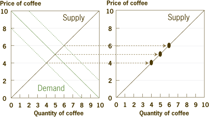
To understand the particular problem mark-up shocks introduce into estimation of the Phillips curve, consider a related estimation problem. Suppose an economist wants to use data on coffee prices and coffee sales to estimate the supply curve for coffee. If the primary type of shock hitting the coffee market is changes in the demand for coffee driven by, say, changes in household income, then the coffee data would reveal an upwardly sloping supply curve, as shifts in the demand for coffee would “trace out” the underlying supply curve. Figure 3 demonstrates this case.

In contrast, if the primary shock hitting the coffee market is changes in supply because of, say, changes in the weather, then the data would trace out the demand curve and a negative relationship! In general, when both types of shocks are buffeting the market, the price-quantity data pairs would resemble a cloud of points, and not a clean supply or a demand relation.

This example shows that the data observed do not necessarily lie along the curve the researcher wants to estimate. There always is a demand curve and a supply curve for coffee, but how do we use data to estimate one versus the other? When we look at the data we see price-quantity pairs that do not easily reveal either the underlying supply or the underlying demand curve. Instead it is an amalgamation of both.

Suppose that a positive relationship between the price and quantity of coffee has been observed historically, but that the relationship has become smaller. That is, an increase in price is now associated with a smaller increase in the quantity of coffee. Does the change reflect a flattening of the supply curve, indicating that the underlying structure of the market has changed, or has the supply curve been hit by more shocks, in which case the structure has not changed? It is difficult to tell these two hypotheses apart.

Because mark-up shocks cause the output gap and inflation to move in opposite directions, they can cause us to mistakenly trace out a negative Phillips curve relationship. Mark-up shocks also hinder economists from correctly identifying the amount of “natural” inflation persistence in the data. Mark-up shocks generate persistent movements in inflation, but only because these shocks generate persistent movements in the gap itself. For a given level of the output gap, inflation will be persistent only if the mark-up shock itself is persistent. Evidence suggests that mark-up shocks are less persistent than the inflation persistence that occurs naturally in the Phillips curve. But if changes in the data are being driven primarily by mark-up shocks, then measured inflation persistence will be lower than the naturally occurring persistence.

The Great Moderation and Inflation Targeting

Our explanation of the effects of mark-up shocks suggests that these shocks might cause economists to estimate a much flatter slope on the Phillips curve and also a lower level of inflation persistence. Whether they will depends not on the absolute level of the mark-up shocks, but on their variability relative to other aggregate shocks such as technology shocks. We do have reason to suspect that the relative importance of mark-up shocks has increased over the period in which we have observed changes in inflation persistence and the curve’s slope.

Looking again at the changes depicted in figure 1, note that the use of 10-year rolling windows means that changes registered in the early 1990s are likely to have originated in the early 1980s. As for what caused these changes, one natural suspect is the sharp decline in output variability (the so-called “Great Moderation”).

Many believe that the Great Moderation which appears to have occurred around the early 1980s was caused largely by a substantial reduction in the variability of technology shocks. The view that the moderation was at least partially due to fewer technology shocks is supported by the fact that total factor productivity, or the amount of output due to factors other than observed changes in capital and labor, has become much less variable since around 1983. Holding fixed the variability of mark-up shocks, the decline in the variability of technology shocks means that mark-up shocks are relatively more important. Hence, the Great Moderation would be consistent with a decrease in observed inflation persistence and the slope of the Phillips curve.

But there was another change that occurred during the early 1980s that could have affected the relative importance of markup shocks on the curve. Central banks around the world began to react more aggressively to inflation than they did in the 1970s. This change might accentuate the effects of mark-up shocks by diminishing the effect of technology shocks on inflation and the gap.

In the absence of an aggressive policy response to movements in inflation, technology shocks expand output and put downward pressure on prices. Because some prices move sluggishly, the downward price pressure is mitigated, and output rises less than potential (that is, the technology shock causes the output gap to decline). An economist trying to estimate the Phillips curve will correctly estimate a positive relationship between inflation and the output gap, as both move in the same direction. An economist would also have little trouble measuring the amount of natural inflation persistence present in the Phillips curve.

But this chain of events would be different in the presence of a monetary policy that attempted to partially stabilize inflation. When the positive technology shock puts downward pressure on inflation, an inflation-targeting central bank will accommodate the extra output generated by expanding the money supply. This expansion increases output toward its potential level, making the gap less volatile as well. In such an environment, technology shocks would have less of an effect on both inflation and the output gap, increasing the relative importance of mark-up shocks. Again, this implies a decline in measured inflation persistence and the slope of the Phillips curve.

No Meaningful Change

Economic theory predicts that the degree of inflation persistence and the slope of the Phillips curve estimated would have dropped since 1983, given the reduction in the importance of technology shocks and greater inflation targeting since that time. These declines, therefore, should not concern policymakers. They do not imply that the sacrifice ratio has changed or that the cost of lowering inflation has risen.