

Household Balance Sheets and the Recovery
Falling home and financial asset prices have combined to weaken the average household’s balance sheet, and this has helped to slow down the current recovery. We examine the role that household balance sheets have typically played in postwar business cycles and assess their importance in explaining why some recoveries, including the current one, have been weaker than others.
The slow pace of the current recovery has been a source of concern for some time. Whereas real GDP growth after severe recessions has generally been very strong, that has not been the case during the current recovery, which followed the worst postwar recession. This time around, it took three years for real GDP to return to where it was just before the start of the recession.
One factor behind the slow recovery has been the weakness of household balance sheets. During the financial crisis, the values of real estate assets and financial assets plunged, lowering household net worth and raising leverage. To repair their balance sheets, households have been increasing their saving rate, raising the average from its pre-recession level of around 2 percent to its current level above 5 percent. This deleveraging process has slowed consumption and, as a result, the recovery.
We examine the role that household balance sheets have played in postwar business cycles and assess their importance in explaining why some recoveries, including the current one, have been weaker than others. We begin by documenting some important differences across past business cycles. We then study the role played by household balance sheets using a simple, conventional model of the U.S. economy. We highlight both the direct impact of balance sheets on economic activity and the indirect mechanism through which balance sheets amplify and propagate the effects of macroeconomic shocks. We find that balance sheets have contributed importantly to the dynamics of some business cycles, especially the more recent ones.
Weaker and Longer Recoveries
Past business cycles have not followed a unique pattern. In particular, there have been important differences in the recoveries. Some recoveries, especially those right after World War II, were strong and rapid. Others, especially the more recent ones, have been weaker and longer.
To compare the different business cycle patterns, we decompose real GDP into the sum of the GDP trend and the GDP gap.1 The trend is determined by long-run factors such as structural productivity, capital accumulation, and long-run growth in the labor force, while the gap is the cyclical component that reflects short-run factors. Since we are interested in business cycle properties, we take the trend as given and base our analysis on the gap.
In the earlier postwar cycles (1948–1960), recoveries were short, rapid, and strong (figure 1). Real GDP rebounded right after the trough of the recession, growing faster than the trend growth rate and rapidly catching up to the trend. The path of the GDP gap was roughly symmetrical around the trough of the recession and looked V-shaped: It first decreased and then rapidly returned to zero, with the recovery phase lasting approximately as long as the recession phase. The two cycles in the 1980s looked V-shaped as well.
Figure 1. Real GDP gap
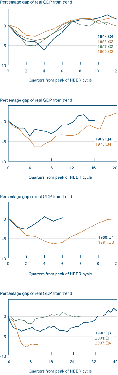
Source: Authors’ calculations from Bureau of Economic Analysis data.
Recoveries were weaker during the 1970s (1969 and 1973 cycles) and they lasted longer—that is, GDP took longer to return to trend. The path of the GDP gap looked more like a check mark than a V, with the recovery phase lasting longer than the recession phase. The longest and weakest recoveries have been the three most recent ones (1990, 2001, and 2007 cycles). There has been no strong GDP rebound or growth, and the recovery phase has lasted years. We might say the path of the GDP gap was somewhat L-shaped, though perhaps it is more accurate to say it was erratic and shapeless.
Another way to see differences in business cycle patterns is by comparing the lengths of recessions with their respective recoveries. Table 1 lists the NBER-measured lengths of all postwar recessions along with two alternative measures for the length of the subsequent recoveries. The first measure is the number of quarters that it took for GDP to return to its trend.
| Cycle | Length of recession (quarters) |
Length of recovery (quarters) |
Duration of recovery (quarters) |
|---|---|---|---|
| D1948:Q4 | 4 | 3 | 1.8834 |
| 1953:Q2 | 4 | 4 | 2.4459 |
| 1957:Q3 | 3 | 4 | 2.2864 |
| 1960:Q2 | 3 | 3 | 2.0014 |
| 1969:Q4 | 4 | 9 | 4.9845 |
| 1973:Q4 | 5 | 13 | 7.3573 |
| 1980:Q1 | 2 | 2 | 1.4951 |
| 1981:Q3 | 5 | 11 | 4.0108 |
| 1990:Q3 | 2 | 32 | 30.7787 |
| 2001:Q1 | 3 | 12 | 10.1975 |
| 2007:Q4 | 6 | >6 | ? |
Source: NBER; authors’ calculations.
The second, which we label the duration of the recovery, is a more sophisticated measure that takes into account whether most of the GDP gap was closed earlier or later during the recovery phase.2
For all the V-shaped business cycles, especially the first four in our sample, the length of the recovery tended not to exceed the length of the preceding recession. In contrast, the recovery lasts longer than the recession in the other business cycles, especially those after 1990.
Not only has the pattern of GDP over the cycle tended to change over time, so has the pattern of unemployment. During the earlier cycles, unemployment peaked approximately at the trough of the recession and then rapidly decreased (figure 2). Since the 1970s, unemployment has peaked later and later and has decreased more slowly.
Figure 2. Unemployment Rate
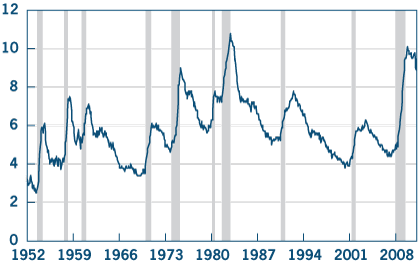
Note: Shaded bars indicate recessions.
Source: Bureau of Economic Analysis.
The Role of Household Balance Sheets
Household balance sheets have been one factor behind these business cycle differences. Balance sheets have been weaker in the slower recoveries.
To measure the weakness of balance sheets, we use leverage, defined as the ratio of assets to net worth. High leverage indicates weak balance sheets. Leverage in the household sector was especially high relative to trend during the 1973, 2001, and 2007 cycles, whose recoveries were especially slow (see figure 3). During all of these three business cycles, financial asset prices experienced sizeable drops. In addition, house prices plunged during the last cycle. As asset prices fell, the value of households’ assets decreased, raising households’ leverage and weakening their balance sheets (a decrease in asset values causes a larger percentage drop in net worth, raising leverage).
Figure 3. Household Leverage
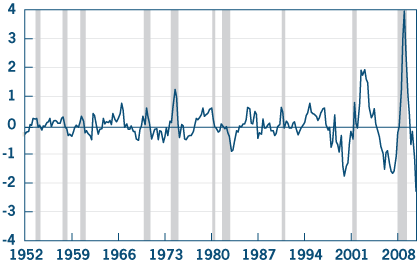
Notes: Leverage is defined as the ratio of assets to net worth. Leverage has been logged and detrended. The trend has been computed using the HP filter. Shaded bars indicate recessions.
Sources: Board of Governors of the Federal Reserve System, Flow of Funds; NBER.
When their leverage is high, households increase their savings because they want to repair their balance sheets. This switch to saving tends to decrease consumption and to slow down the recovery. In fact, data show that leverage relative to trend is negatively correlated with present and future production, so high leverage tends to be associated with and followed by a decrease in real activity. This type of evidence is not sufficient by itself to identify the role played by household balance sheets in business cycles, however. It can show that high leverage is associated with low economic activity, but it cannot discern whether leverage actively causes changes in economic activity or whether it passively responds to economic activity.
To formally assess the relationship between balance sheets and the business cycle, we use a common, simple model of the aggregate economy. The variables included are production, the unemployment rate, inflation, the short-term risk-free interest rate, an oil-price index, and household leverage. The model, a vector auto-regression (VAR), relates each variable to the past values of all variables in the model and to various types of shocks.3 This type of model has been shown to effectively capture the dynamics of the business cycle—we use it to determine how changes in balance sheets affect economic activity and how balance sheets respond to changes in the economy.
First, we look at the economic effects of a shock to balance sheets, that is, an unanticipated increase in leverage. For instance, an adverse balance sheet shock could be the result of an unexpected drop in the price of real estate or financial assets. Our model suggests that the response of the economy to such a shock is the one we would expect based on intuition: After an unanticipated increase in leverage, real GDP decreases and unemployment increases (figures 4 and 5). So adverse balance sheet shocks discourage economic activity. Moreover, the responses of real GDP and unemployment are delayed and persistent, with the peak of the responses not occurring until approximately a year or more after the shock hits. In contrast, the responses of real GDP and unemployment to shocks that affect them directly are more immediate: The peaks of the responses occur after only one and two quarters, respectively. This suggests that balance sheet shocks cause important changes in economic activity and that their effect is more delayed than that of other shocks.
Figure 4. Response of Real GDP to Two Contractionary Shocks
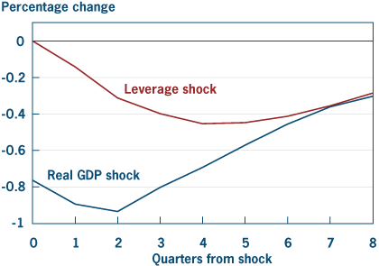
Note: This figure plots the impulse response functions of real GDP to macroeconomic and balance sheet shocks. The impulse response function tracks the average response over time to a shock occurring in period zero. It is the deviation in the path that a variable follows over time due to the occurrence of the shock. The size of the shock is equal to its average size in the time period considered (one standard deviation). Responses are statistically significant at a 5 percent level for two years.
Source: Authors’ calculations.
Figure 5. Response of the Unemployment Rate to Two Contractionary Shocks
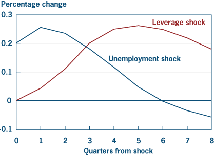
Note: This figure plots the impulse response functions of unemployment to macroeconomic and balance sheet shocks. The impulse response function tracks the average response over time to a shock occurring in period zero. It is the deviation in the path that a variable follows over time due to the occurrence of the shock. The size of the shock is equal to its average size in the time period considered (one standard deviation). The response to an unemployment shock is statistically significant at a 5 percent level for five quarters, while the response to a balance sheet shock is statistically significant for two and a half years.
Source: Authors’ calculations.
We also use the VAR to evaluate the relative contribution of balance sheet shocks and other shocks to business cycles. For each business cycle, we took the path that was expected for GDP at the beginning of the cycle, looked at the deviation from the path over the cycle, and decomposed the deviation into the part due to balance sheet shocks and the part due to all other shocks. This decomposition reveals that adverse balance sheet shocks played an important role in three cycles—1973, 1990, and especially 2007, the most recent one (figure 6). Balance sheet shocks caused real GDP to be below its expected path by 3.8 percentage points in the fourth quarter of 2009, accounting for 84 percent of the total drop. They were important during the recovery phase of the 2001 cycle as well. The decomposition for unemployment leads to very similar conclusions. Since balance sheet shocks tend to have a more delayed effect on economic activity relative to other shocks, this explains in part why the later recoveries have been slower.
Figure 6. Contribution of balance sheet shocks to business cycles
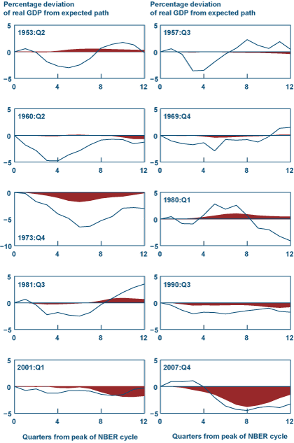
Notes: For each business cycle episode, we plot the deviation of real GDP from its path expected at the beginning of the cycle (solid line). This deviation is due to all types of shocks hitting the economy (including balance sheet shocks). The shaded area shows the portion of the deviation of real GDP from its expected path that is due to balance sheet shocks only.
Source: Authors’ calculations.
Our results so far have highlighted the importance of the direct impact of balance sheets shocks on economic activity. However, balance sheets play another important role: They amplify and propagate the effects of macroeconomic shocks. After an adverse macroeconomic shock, an increase in leverage reinforces the direct contractionary effect of the shock.
To study whether this indirect mechanism can explain part of differences in business cycle patterns, we consider separately the two periods before and after 1985, estimating the VAR model separately for the two periods (figure 7). This reveals that the response of leverage to macroeconomic shocks has changed over time. In response to a contractionary shock to GDP, such as an adverse productivity shock, leverage tended to decrease before 1985, thereby attenuating the effects of the shock, while it has tended to increase after 1985, thereby amplifying and propagating the effects of the shock. As a result of this change, balance sheets have deteriorated more in response to contractionary macroeconomic shocks after 1985, and this development is likely to have contributed to slowing down the later recoveries.
Figure 7. Response of leverage to a contractionary GDP shock before and after 1985
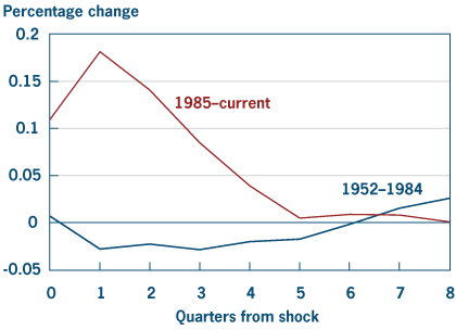
Notes: Response to a one-standard-deviation shock. The response of leverage is not statistically significant at a 5 percent level before 1985, whereas it is statistically significant for two quarters in the period after 1985.
Source: Authors’ calculations.
Conclusion
By using fairly conventional methods and assumptions, we have unveiled some general patterns. We have found that weak household balance sheets have been an important factor behind the slower recoveries, especially the current one. One reason is that balance sheet shocks, which tend to have a delayed and persistent effect on economic activity, have played a greater role in the cycles associated with the slower recoveries. Another reason is that since about 1985, balance sheets have deteriorated more in response to adverse macroeconomic shocks than they used to, and as a result they have amplified and propagated the direct contractionary effects of the shocks.
Because the VAR model that we have used is a simplified representation of the economy, it will be important to confirm our results using more sophisticated models. Also, we have documented the differing impacts of household balance sheets in different business cycles, but we haven’t examined the reasons behind those differing impacts. One possibility could be, for instance, that changes in the types of assets and liabilities that households have on their balance sheets—and their greater sensitivities to asset price shocks—might have something to do with both the greater role played by balance sheet shocks and the different response of leverage to macroeconomic shocks in the later cycles.
When our results are used to interpret recent evidence on household finances, they suggest conditions may be improving. While households have been saving at a high rate to repair their balance sheets for some time, there have been signs that this deleveraging process has attenuated: Household leverage has come down from its peak and the saving rate has leveled out. These signs may point to a stronger pickup of consumption and a more robust recovery.
Footnotes
- More precisely, we decompose the logarithm of real GDP into the sum of its trend and the log-GDP gap. In turn, we compute the log-GDP trend as the piecewise linear trend that interpolates the NBER peaks of log-GDP. For the 1960:Q2 cycle, however, the resulting trend growth would be too high and would distort the results, so we use the average postwar growth rate instead. For the last cycle (2007:Q4), we extend the trend line from the previous 2001:Q1 cycle. Return
- The duration of the recovery is the weighted average of the number of quarters that it took for GDP to return to its trend. To construct the average, each quarter is weighted by the percentage of the total GDP gap that was closed in that quarter. For instance, if 1/3 of the GDP gap were closed in the first quarter of the recovery, and 2/3 in the second quarter, the duration would be (1/3 x 1) + (2/3 x 2) = 5/3 = 1.66 quarters. Return
- The model is a four-lag VAR of the following variables: the log of real GDP, the unemployment rate, the log of the GDP price deflator, the three-month T-bill rate, the log of the WTI oil price, and the log of household leverage for the period 1952:Q1–2010:Q2. Shocks are identified using a Cholesky decomposition with the variables ordered as listed above. Return
The views authors express in Economic Commentary are theirs and not necessarily those of the Federal Reserve Bank of Cleveland or the Board of Governors of the Federal Reserve System. The series editor is Tasia Hane. This work is licensed under a Creative Commons Attribution-NonCommercial 4.0 International License. This paper and its data are subject to revision; please visit clevelandfed.org for updates.
Suggested Citation
Bianco, Timothy, and Filippo Occhino. 2011. “Household Balance Sheets and the Recovery.” Federal Reserve Bank of Cleveland, Economic Commentary 2011-05. https://doi.org/10.26509/frbc-ec-201105
This work by Federal Reserve Bank of Cleveland is licensed under Creative Commons Attribution-NonCommercial 4.0 International


- Share